Linear predictive models for bitcoin price

The most extreme form of linear predictive models is one in which all the coefficients are equal in magnitude (but not necessarily in sign). For example, suppose you have identified a number of factors ( $f^{\prime}$ s) that are useful in predicting whether tomorrow’s return of a bitcoin index is positive. One factor may be today’s return, with a positive today’s return predicting a positive future return. Another factor may be today’s change in the volatility index (VIX), with a negative change predicting positive future return. You may have several such factors. If you normalize these factors by turning them first into Z-scores (using in-sample data!):
$$
z(i)=(f(i)-\operatorname{mean}(f)) / \operatorname{std}(f)
$$
where $f(i)$ is the $i^{\text {th }}$ factor, you can then predict tomorrow’s return $R$ by
$$
R=\operatorname{mean}(R)+\operatorname{std}(R) \sum_{i}^{n} \operatorname{sign}(i) z(i) / n
$$
The quantities mean $(f)$ and $s t d(f)$ are the historical average and standard deviation of the various $f(i),$ sign $(i)$ is the sign of the historical correlation between $f(i)$ and $R,$ and $\operatorname{mean}(R)$ and $s t d(R)$ are the historical average and

Statistical Significance of Backtesting:
Hypothesis Testing

In any backtest, we face the problem of finite sample size: Whatever statistical measures we compute, such as average returns or maximum drawdowns, are subject to randomness. In other words, we may just be lucky that our strategy happened to be profitable in a small data sample. Statisticians have developed a general methodology called hypothesis testing to address this issue.

The general framework of hypothesis testing as applied to backtesting follows these steps:

Based on a backtest on some finite sample of data, we compute a certain statistical measure called the test statistic. For concreteness, let’s say the test statistic is the average daily return of a trading strategy in that period.
We suppose that the true average daily return based on an infinite data set is actually zero. This supposition is called the null hypothesis.
We suppose that the probability distribution of daily returns is known. This probability distribution has a zero mean, based on the null hypothesis. We describe later how we determine this probability distribution.
Based on this null hypothesis probability distribution, we compute the probability $p$ that the average daily returns will be at least as large as the observed value in the backtest (or, for a general test statistic, as extreme, allowing for the possibility of a negative test statistic). This probability $p$ is called the p-value, and if it is very small (let’s say smaller than 0.01), that means we can “reject the null hypothesis,” and conclude that the backtested average daily return is statistically signifi cant.

The step in this procedure that requires most thought is step $3 .$ How do we determine the probability distribution under the null hypothesis? Perhaps we can suppose that the daily returns follow a standard parametric probability distribution such as the Gaussian distribution, with a mean of zero and a standard deviation given by the sample standard deviation of the daily returns. If we do this, it is clear that if the backtest has a high Sharpe ratio, it would be very easy for us to reject the null hypothesis. This is because the standard test statistic for a Gaussian distribution is none other than the average divided by the standard deviation and multiplied by the square root of the number of data points (Berntson, 2002$)$. The $p$ -values for various critical values are listed in Table $1.1 .$ For example, if the daily Sharpe ratio multiplied by the square root of the number days $(\sqrt{n})$ in the backtest is greater than or equal to the critical value $2.326,$ then the $p$ -value is smaller than or equal to 0.01 .

But this is actually just a stopgap measure. In fact, if the difficulty of obtaining real data in the trading market is greatly reduced, then reinforcement learning based on reinforcement learning will show considerable power

The Basics of Mean Reversion

Is mean reversion also prevalent in fi nancial price series? If so, our lives as
traders would be very simple and profi table! All we need to do is to buy low
(when the price is below the mean), wait for reversion to the mean price,
and then sell at this higher price, all day long. Alas, most price series are
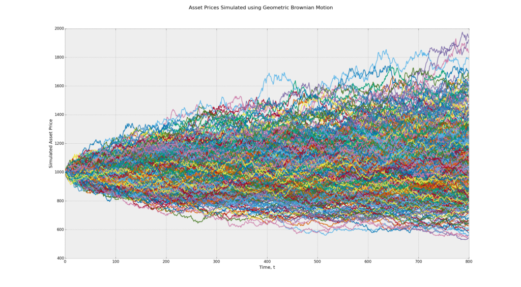
not mean reverting, but are geometric random walks.

The returns, not the prices, are the ones that usually randomly distribute around a mean of zero.
Unfortunately, we cannot trade on the mean reversion of returns. (One
should not confuse mean reversion of returns with anti-serial-correlation
of returns, which we can defi nitely trade on. But anti-serial-correlation of
returns is the same as the mean reversion of prices.) Those few price series
that are found to be mean reverting are called stationary, and in this chapter
we will describe the statistical tests (ADF test and the Hurst exponent and
Variance Ratio test) for stationarity. There are not too many prefabricated

Augmented Dickey-Fuller Test

If a price series is mean reverting, then the current price level will tell us something about what the price’s next move will be: If the price level is higher than the mean, the next move will be a downward move; if the price level is lower than the mean, the next move will be an upward move. The ADF test is based on just this observation. We can describe the price changes using a linear model:
$$
\Delta y(t)=\lambda y(t-1)+\mu+\beta t+\alpha_{1} \Delta y(t-1)+\cdots+\alpha_{k} \Delta y(t-k)+\epsilon_{t}
$$
where $\Delta y(t) \equiv y(t)-y(t-1), \Delta y(t-1) \equiv y(t-1)-y(t-2),$ and so on. The ADF
test will find out if $\lambda=0$. If the hypothesis $\lambda=0$ can be rejected, that means the next move $\Delta y(t)$ depends on the current level $y(t-1),$ and therefore it is not a random walk. The test statistic is the regression coefficient $\lambda$ (with $y(t-1)$ as the independent variable and $\Delta y(t)$ as the dependent variable) divided by the standard error of the regression fit: $\lambda / \mathrm{SE}(\lambda)$. The statisticians Dickey and Fuller have kindly found out for us the distribution of this test statistic and tabulated the critical values for us, so we can look up for any value of $\lambda / \operatorname{SE}(\lambda)$ whether the hypothesis can be rejected at, say, the 95 percent probability level.

Notice that since we expect mean regression, $\lambda / \mathrm{SE}(\lambda)$ has to be negative, and it has to be more negative than the critical value for the hypothesis to be rejected. The critical values themselves depend on the sample size and whether we assume that the price series has a non-zero mean $-\mu / \lambda$ or a steady drift $-\beta t / \lambda .$ In practical trading, the constant drift in price, if any, tends to be of a much smaller magnitude than the daily fluctuations in price. So for simplicity we will assume this drift term to be zero $(\beta=0)$.

Kalman Filter as Market-Making Model

Kalman Filter is very poupular in SLAM, in fact it is almost near the perfect in some simple situaiton. the adventage of SLAM than finance market is the state space is much more predictable, or in other word the non-zero value of the transition matrix is much more cancertrate.

There is an application of Kalman filter to a meanreverting strategy. In this application we are concerned with only one mean-reverting price series; we are not concerned with finding the hedge ratio between two cointegrating price series. However, we still want to find the mean price and the standard deviation of the price series for our mean reversion trading. So the mean price $m(t)$ is the hidden variable here, and the price $y(t)$ is the observable variable. The measurement equation in this case is trivial:
$$
y(t)=m(t)+\epsilon(t)
$$
(“Measurement equation”)
with the same state transition equation
$$
m(t)=m(t-1)+\omega(t-1)
$$
(“State transition”)
So the state update equation is just
$$
m(t \mid t)=m(t \mid t-1)+K(t)(y(t)-m(t \mid t-1)) . \quad(\text { “State update” })
$$
(This may be the time to review Box 3.1 if you skipped it on first reading.) The variance of the forecast error is
$$
Q(t)=\operatorname{Var}(m(t))+V_{e}
$$
The Kalman gain is
$$
K(t)=R(t \mid t-1) /\left(R(t \mid t-1)+V_{e}\right)
$$
and the state variance update is
$$
R(t \mid t)=(1-K(t)) R(t \mid t-1)
$$

Why are these equations worth highlighting? Because this is a favorite model for market makers to update their estimate of the mean price of an asset, as Euan Sinclair pointed out (Sinclair, 2010$)$. To make these equations more practical, practitioners make further assumptions about the measurement error $V_{e}$, which, as you may recall, measures the uncertainty of the observed transaction price. But how can there be uncertainty in the observed transaction price? It turns out that we can interpret the uncertainty in such a way that if the trade size is large (compared to some benchmark), then the uncertainty is small, and vice versa. So $V_{e}$ in this case becomes a function of $t$ as well. If we denote the trade size as $T$ and the benchmark trade size as $T_{\max }$, then $V_{e}$ can have the form
$$
V_{e}=R(t \mid t-1)\left(\frac{T}{T_{\max }}-1\right)
$$
So you can see that if $T=T_{\max },$ there is no uncertainty in the observed price, and the Kalman gain is $1,$ and hence the new estimate of the mean price $m(t)$ is exactly equal to the observed price! But what should $T_{\max }$ be? It can be some fraction of the total trading volume of the previous day, for example, where the exact fraction is to be optimized with some training data. Note the similarity of this approach to the so-called volume-weighted average price (VWAP) approach to determine the mean price, or fair value of an asset. In the Kalman filter approach, not only are we giving more weights to trades with larger trade sizes, we are also giving more weights to more recent trade prices. So one might compare this to volume and timeweighted average price.

Interday Momentum Strategies

There are four main causes of momentum:

For futures, the persistence of roll returns, especially of their signs.
The slow diff usion, analysis, and acceptance of new information.
The forced sales or purchases of assets of various type of funds.
Market manipulation by high-frequency traders.

We will be discussing trading strategies that take advantage of each cause
of momentum in this and the next chapter. In particular, roll returns of futures,
which featured prominently in the last chapter, will again take center
stage. Myriad futures strategies can be constructed out of the persistence of
the sign of roll returns

Nonoverlapping Periods for Correlation Calculations

With the advent of machine-readable, or “elementized,” news feeds, for example, Aicoin use Twitter API, it is now
possible to programmatically capture all the news items on a company, not
just those that fit neatly into one of the narrow categories such as earnings
announcements or merger and acquisition (M&A) activities. Furthermore,
natural language processing algorithms are now advanced enough to analyze
the textual information contained in these news items, and assign a “sentiment
score” to each news article that is indicative of its price impact on a
bitcoin market, and an aggregation of these sentiment scores from multiple news articles
from a certain period was found to be predictive of its future return.
For example, Hafez and Xie, using RavenPack’s Sentiment Index, found that
buying a portfolio of bitcoin with positive sentiment change and shorting
one with negative sentiment change results in an APR from 52 percent to
156 percent and Sharpe ratios from 3.9 to 5.3 before transaction costs, depending
on how many bitcoin are included in the portfolios (Hafez and Xie,
2012). The success of these cross-sectional strategies also demonstrates very
neatly that the slow diffusion of news is the cause ofbitcoin momentum.
There are other vendors besides RavenPack that provide news sentiments
on bitcoin. If you believe your own sentiment algorithm is better than
theirs, you can subscribe directly to an element-sized news feed instead
and apply your algorithm to it. I mentioned before that Newswire offers
a low-cost version of this type of news feeds, but offerings with lower
latency and better coverage are provided by Bloomberg Event-Driven

Kelly formula

If the probability distribution of returns is Gaussian distribution, the Kelly formula gives us a very simple answer for optimal leverage $f$ :
$$
f=m / s^{2}
$$
where $m$ is the mean excess return, and $s^{2}$ is the variance of the excess
returns.

The best expositions of this formula can be found in the summary paper, Edward Thorp’s (1997) paper, in fact, it can be proven that if the Gaussian assumption is a good approximation, then the Kelly leverage $f$ will generate the highest compounded growth rate of equity, assuming that all profits are reinvested. However, even if the Gaussian assumption is really valid, we will inevitably suffer estimation errors when we try to estimate what the “true” mean and variance of the excess return are. And no matter how good one’s estimation method is, there is no guarantee that the future mean and variance will be the same as the historical ones. The consequence of using an overestimated mean or an underestimated variance is dire: Either case will lead to an overestimated optimal leverage, and if this overestimated leverage is high enough, it will eventually lead to ruin: equity going to zero. However, the consequence of using an underestimated leverage is merely a submaximal compounded growth rate. Many traders justifiably prefer the later scenario, and they routinely deploy leverage equal to half of what the Kelly formula recommends: the so-called half-Kelly leverage.

There is another usage of the Kelly formula besides setting the optimal leverage: it also tells us how to optimally allocate our buying power to different portfolios or strategies. Let’s denote $F$ as a column vector of optimal leverages that we should apply to the different portfolios based on a common pool of equity. (For example, if we have $\$ 1$ equity, then $F=[3.21 .5]^{T}$ means the first portfolio should have a market value of $\$ 3.2$ while the second portfolio should have a market value of $\$ 1.5$. The $T$ signifies matrix transpose.) The Kelly formula says
$$
F=C^{-1} M
$$