统计代写| Matrix calculations stat代写
统计代考
$11.6 \mathrm{R}$
Matrix calculations
Let’s do some calculations for the 4-state Markov chain in Example 11.1.5, as an example of working with transition matrices in R. First, we need to specify the transition matrix $Q$. This is done with the matrix command: we type in the entries
522
of the matrix, row by row, as a long vector, and then we tell $\mathrm{R}$ the number of rows and columns in the matrix (nrow and ncol), as well as the fact that we typed in the entries by row (byrow=TRUE):
$Q<-\operatorname{matrix}(c(1 / 3,1 / 3,1 / 3,0,$,
$$
\begin{aligned}
&(1 / 3,1 / 3,1 / 3,0, \
&0,0,1 / 2,1 / 2, \
&0,1,0,0, \
&1 / 2,0,0,1 / 2), \mathrm{nrow}=4, \mathrm{ncol}=4, \text { byrow=TRUE) }
\end{aligned}
$$
To obtain higher order transition probabilities, we can multiply $Q$ by itself repeatedly. The matrix multiplication command in $\mathrm{R}$ is $\% * \%$ (not just *). So
$Q 2<-Q \% * \%$
$Q 3<-Q 2 \% * \%$
$Q 4<-Q 2 \% * \%$ Q 2
Q5 <- Q3 \%*\% Q2
produces $Q^{2}$ through $Q^{5}$. If we want to know the probability of going from state 3 to state 4 in exactly 5 steps, we can extract the $(3,4)$ entry of $Q^{5}$ :
Q5 $[3,4]$
This gives $0.229$, agreeing with the value $11 / 48$ shown in Example 11.1.5. can use the command $Q \% \% \mathrm{n}$ after installing and loading the expm package. For example, $Q \%^{\sim} \%$ yields $Q^{42}$. By exploring the behavior of $Q^{n}$ as $n$ grows, we can see Theorem 11.3.6 in action (and get a sense of how long it takes for the chain to get very close to its stationary distribution).
In particular, for $n$ large each row of $Q^{n}$ is approximately $(0.214,0.286,0.214,0.286)$, so this is approximately the stationary distribution. Another way to obtain the stationary distribution numerically is to use
eigen $(t(Q))$
to compute the eigenvalues and eigenvectors of the transpose of $Q$; then the eigenvector corresponding to the eigenvalue 1 can be selected and normalized so that the components sum to $1 .$
Gambler’s ruin
To simulate from the gambler’s ruin chain from Example $11.2 .6$, we start by deciding the total amount of money $\mathbb{N}$, the probability $p$ of gambler $A$ winning a given round, and the number of time periods nsim that we wish to simulate.
$\mathrm{N}<-10$
$\mathrm{p}<-1 / 2$
nsim <- 80
统计代考
$11.6 \mathrm{R}$
矩阵计算
让我们对示例 11.1.5 中的 4 状态马尔可夫链进行一些计算,作为在 R 中使用转移矩阵的示例。首先,我们需要指定转移矩阵 $Q$。这是通过矩阵命令完成的:我们输入条目
522
矩阵,逐行,作为一个长向量,然后我们告诉 $\mathrm{R}$ 矩阵中的行数和列数(nrow 和 ncol),以及我们输入条目的事实按行(byrow=TRUE):
$Q<-\operatorname{矩阵}(c(1 / 3,1 / 3,1 / 3,0,$,
$$
\开始{对齐}
&(1 / 3,1 / 3,1 / 3,0, \
&0,0,1 / 2,1 / 2, \
&0,1,0,0, \
&1 / 2,0,0,1 / 2), \mathrm{nrow}=4, \mathrm{ncol}=4, \text { byrow=TRUE) }
\end{对齐}
$$
为了获得更高阶的转移概率,我们可以重复地将 $Q$ 与自身相乘。 $\mathrm{R}$ 中的矩阵乘法命令是 $\% * \%$(不仅仅是 *)。所以
$Q 2<-Q \% * \%$
$Q 3<-Q 2 \% * \%$
$Q 4<-Q 2 \% * \%$ Q 2
Q5 <- Q3 \%*\% Q2
通过 $Q^{5}$ 产生 $Q^{2}$。如果我们想知道在恰好 5 步内从状态 3 到状态 4 的概率,我们可以提取 $Q^{5}$ 的 $(3,4)$ 条目:
第五季度 $[3,4]$
这给出了 $0.229$,与示例 11.1.5 中显示的值 $11 / 48$ 一致。安装并加载 expm 包后可以使用命令 $Q \% \% \mathrm{n}$。例如,$Q \%^{\sim} \%$ 产生 $Q^{42}$。通过探索 $Q^{n}$ 随着 $n$ 增长的行为,我们可以看到定理 11.3.6 的作用(并了解链需要多长时间才能非常接近其平稳分布)。
特别是,对于 $n$ 大,$Q^{n}$ 的每一行大约是 $(0.214,0.286,0.214,0.286)$,所以这近似于平稳分布。另一种以数值方式获得平稳分布的方法是使用
特征 $(t(Q))$
计算$Q$转置的特征值和特征向量;然后可以选择特征值 1 对应的特征向量并对其进行归一化,使得分量总和为 $1 .$
赌徒的废墟
为了模拟示例 $11.2 .6$ 中赌徒的破产链,我们首先确定总金额 $\mathbb{N}$、赌徒 $A$ 赢得给定回合的概率 $p$ 以及我们希望模拟的时间段 nsim。
$\mathrm{N}<-10$
$\mathrm{p}<-1 / 2$
nsim <- 80
。
R语言代写

统计代写|SAMPLE SPACES AND PEBBLE WORLD stat 代写 请认准UprivateTA™. UprivateTA™为您的留学生涯保驾护航。