物理代写| Curvature 相对论代考
物理代写
sports a vector over a closed loop, the vector d4.5 Curvature
Curvature is a key property of a multi-dimensional space. It is an intrinsic property of space, which cannot be removed by coordinate transformations. We will see later, that gravity manifests itself as curvature in space-time, so the measurement of curvature is very important for the understanding of gravitation.
Measurement of curvature is not a trivial task. For a long time humans used to think that the earth is flat-flat like a circular disc! When it comes to Earth, our perception of the “vertical” dimension is much smaller compared to the radius of the earth; in this case we are like very small ants on a football who can only see along the ball’s surface. In general, to understand gravity, we need to deal with the curvature of $3+1$ dimensional space-time, which is impossible to visualise. One cannot even visualise a three sphere, because our brain cannot perceive more than three dimensions.
We ask the question could an ant draw the conclusion that the surface of a sphere is curved by making measurements entirely within the sphere. The answer is yes. The ant could draw a small circle on the sphere and measure its radius along the surface of the sphere and also its circumference. It will find the circumference to radius ratio is less than $2 \pi$. It will find that the ratio falls short by the factor $1-r^{2} / 6 R^{2}$, upto second order in $r / R$, where $r$ is the radius of the circle, measured along the surface of the sphere, and $R$ is the radius of the sphere. The quantity $K=1 / R^{2}$ is known as the Gaussian curvature. For a general surface the formula generalises to $1-K r^{2} / 6$. This kind of curvature is called the intrinsic curvature because it has been obtained by making measurements entirely within the surface. The other kind of curvature is the extrinsic curvature when the surface is embedded in a three dimensional space, usually Euclidean space. In GR we are interested in the intrinsic curvature of the 4 dimensional spacetime. The Gaussian curvature which is defined for 2-surfaces is intimately connected with the Riemann curvature tensor.
4.5.1 Riemann-Christoffel Curvature Tensor
A key indicator of curvature is that if one parallel transports a vector over a closed loop, the vector does not return to its original orientation. This can be illustrated by performing the following exercise on a two
sphere (See Exercise 4.2). A vector parallely transported around a latitude
(except the equator) does not return to itself,oes not return to its original
orientation. This can be illustrated by performing the following exercise on a
two sphere (See Exercise 4.2). A vector parallely transported around a
latitude (except the equator) does not return to itself,
A key indicator of curvature is that if one parallel transports a vector over a closed loop, the vector does not return to its original orientation. This can be illustrated by performing the following exercise on a two sphere (See Exercise 4.2). A vector parallely transported around a latitude (except the equator) does not return to itself,
$4.5$ Curvature
77
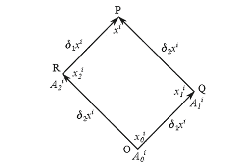
Fig. 4.2 Parallel transport over a closed loop does not bring a vector back to the original orientation. The final difference in orientation, in fact, provides a measure of curvature. A vector $\mathbf{A}{\mathbf{0}} \equiv A{0}^{i}$ is parallel transported from point $\mathrm{O}$ to $\mathrm{P}$ via points $\mathrm{Q}$ and $\mathrm{R}$. The result is not the same in general-it is path dependent. The difference between the parallely transported vectors measures the curvature, namely, the relevant component of the Riemann tensor
showing that the sphere posseses non-zero curvature or the sphere is a curved space. If one has to measure the curvature at a given point in space, one would construct an infinitesimal closed loop around that point and parallel transport a vector around the loop, the change in the vector is directly related to the measure of curvature.
Let us consider a vector $\mathbf{A}{0} \equiv A{0}^{i}$ parallelly transported around the closed rectangle OQPRO, bounded by infinitesimal displacements $\delta_{1} x^{i}, \delta_{2} x^{i},-\delta_{1} x^{i}$ and $-\delta_{2} x^{i}$ respectively. The procedure is depicted in Fig. 4.2. To the leading order, this equals the difference between the value of the vector at $\mathrm{P}$ if it was transported from $\mathrm{O}$ via Q versus via R. That is, parallel transport is path dependent, the transported vector components depend on the path taken.
The difference $\Delta A^{i}$ via two different paths can be calculated. Let us first take path 1 and transport $A_{0}^{i}$ from $O$ to $Q$. We then have:
$$
\begin{aligned}
\delta A_{O \rightarrow Q}^{i} &=-\Gamma^{i}{ }{j k}(O) A{0}^{j} \delta_{1} x^{k}, \
A^{i}(Q) &=A_{0}^{i}+\delta A_{O \rightarrow Q}^{i}=A_{0}^{i}-\Gamma^{i}{ }{j k}(O) A{0}^{j} \delta_{1} x^{k},
\end{aligned}
$$
where the Christoffel symbols are evaluated at $O$. Further parallely transport $A^{i}(Q)$ to $P$ to obtain $A^{i}(P) \equiv A_{1}^{i}$ in a similar way. We then have,
$$
A_{1}^{i}=A^{i}(Q)-\Gamma_{j k}^{i}(Q) A^{j}(Q) \delta_{2} x^{k},
$$
where now the Chrisoffel symbols are evaluated at $Q$. We now Taylor expand the Christoffel symbols to first order around $O$ to obtain their values at $Q$ approximately:
物理代考
在闭环上运动一个向量,向量 d4.5 曲率
曲率是多维空间的关键属性。它是空间的固有属性,不能通过坐标变换消除。稍后我们会看到,引力在时空中表现为曲率,所以曲率的测量对于理解引力非常重要。
曲率的测量并非易事。长期以来,人类一直认为地球是平平的,就像一个圆盘!说到地球,与地球的半径相比,我们对“垂直”维度的感知要小得多;在这种情况下,我们就像足球上的小蚂蚁,只能看到球的表面。一般来说,要理解引力,我们需要处理 $3+1$ 维时空的曲率,这是无法想象的。一个人甚至无法想象三个球体,因为我们的大脑不能感知超过三个维度。
我们问一个问题,蚂蚁能否通过完全在球体内进行测量得出球体表面是弯曲的结论。答案是肯定的。蚂蚁可以在球体上画一个小圆圈,并沿着球体的表面测量它的半径以及它的周长。它会发现周长比小于$2 \pi$。它将发现该比率低于 $1-r^{2} / 6 R^{2}$ 的因子,达到 $r / R$ 的二阶,其中 $r$ 是圆的半径,沿测量球的表面,$R$ 是球的半径。量 $K=1 / R^{2}$ 称为高斯曲率。对于一般曲面,该公式推广到 $1-K r^{2} / 6$。这种曲率被称为固有曲率,因为它是通过完全在表面内进行测量而获得的。另一种曲率是曲面嵌入三维空间(通常是欧几里得空间)时的外曲率。在 GR 中,我们对 4 维时空的内在曲率感兴趣。为 2 面定义的高斯曲率与黎曼曲率张量密切相关。
4.5.1 Riemann-Christoffel 曲率张量
曲率的一个关键指标是,如果一个平行线在闭环上传输矢量,则该矢量不会返回其原始方向。这可以通过在两个
球体(见练习 4.2)。绕纬度平行传输的向量
(除赤道外)不回归本源,不回归本源
方向。这可以通过执行以下练习来说明
两个球体(见练习 4.2)。一个向量在一个周围平行传输
纬度(赤道除外)不返回自身,
曲率的一个关键指标是,如果一个平行线在闭环上传输矢量,则该矢量不会返回其原始方向。这可以通过在两个球体上执行以下练习来说明(参见练习 4.2)。绕纬度(赤道除外)平行传输的矢量不会返回自身,
$4.5$ 曲率
77
图 4.2 闭环上的并行传输不会将矢量带回原始方向。事实上,最终的方向差异提供了曲率的度量。向量 $\mathbf{A}{\mathbf{0}} \equiv A{0}^{i}$ 通过点 $ 从 $\mathrm{O}$ 到 $\mathrm{P}$ 并行传输\mathrm{Q}$ 和 $\mathrm{R}$。结果通常是不一样的——它是路径相关的。平行传输向量之间的差异测量曲率,即黎曼张量的相关分量
表明球体具有非零曲率或球体是弯曲空间。如果必须测量空间中给定点的曲率,可以围绕该点构建一个无限小的闭环,并在该环周围平行传输一个向量,向量的变化与曲率的测量直接相关。
让我们考虑一个向量 $\mathbf{A}{0} \equiv A{0}^{i}$ 围绕闭合矩形 OQPRO 并行传输,以无穷小的位移 $\delta_{1} x^{i} 为界, \delta_{2} x^{i},-\delta_{1} x^{i}$ 和 $-\delta_{2} x^{i}$。该过程如图 4.2 所示。对于领先的顺序,这等于向量在 $\mathrm{P}$ 处的值之间的差,如果它是从 $\mathrm{O}$ 通过 Q 与通过 R 传输的。也就是说,并行传输是路径相关的,传输的矢量分量取决于所采用的路径。
可以计算出两条不同路径的差值$\Delta A^{i}$。让我们首先采用路径 1 并将 $A_{0}^{i}$ 从 $O$ 传输到 $Q$。然后我们有:
$$
\开始{对齐}
\delta A_{O \rightarrow Q}^{i} &=-\Gamma^{i}{ }{jk}(O) A{0}^{j} \delta_{1} x^{k}, \
A^{i}(Q) &=A_{0}^{i}+\delta A_{O \rightarrow Q}^{i}=A_{0}^{i}-\Gamma^{i}{ } {jk}(O) A{0}^{j} \delta_{1} x^{k},
\end{对齐}
$$
克里斯托弗符号在哪里

物理代考Gravity and Curvature of Space-Time 代写 请认准UprivateTA™. UprivateTA™为您的留学生涯保驾护航。
电磁学代考
物理代考服务:
物理Physics考试代考、留学生物理online exam代考、电磁学代考、热力学代考、相对论代考、电动力学代考、电磁学代考、分析力学代考、澳洲物理代考、北美物理考试代考、美国留学生物理final exam代考、加拿大物理midterm代考、澳洲物理online exam代考、英国物理online quiz代考等。
光学代考
光学(Optics),是物理学的分支,主要是研究光的现象、性质与应用,包括光与物质之间的相互作用、光学仪器的制作。光学通常研究红外线、紫外线及可见光的物理行为。因为光是电磁波,其它形式的电磁辐射,例如X射线、微波、电磁辐射及无线电波等等也具有类似光的特性。
大多数常见的光学现象都可以用经典电动力学理论来说明。但是,通常这全套理论很难实际应用,必需先假定简单模型。几何光学的模型最为容易使用。
相对论代考
上至高压线,下至发电机,只要用到电的地方就有相对论效应存在!相对论是关于时空和引力的理论,主要由爱因斯坦创立,相对论的提出给物理学带来了革命性的变化,被誉为现代物理性最伟大的基础理论。
流体力学代考
流体力学是力学的一个分支。 主要研究在各种力的作用下流体本身的状态,以及流体和固体壁面、流体和流体之间、流体与其他运动形态之间的相互作用的力学分支。
随机过程代写
随机过程,是依赖于参数的一组随机变量的全体,参数通常是时间。 随机变量是随机现象的数量表现,其取值随着偶然因素的影响而改变。 例如,某商店在从时间t0到时间tK这段时间内接待顾客的人数,就是依赖于时间t的一组随机变量,即随机过程