
数学代写| The Decision Space: m × 2 Problems 凸优化代考
凸优化代写
We now discuss techniques for solving linear programming problems. In general, methods of solution involving graphs and pictures are limited to small problems. The most well-known method works for problems with only two decision variables, but there is no limit on the number of constraints; in other words, it works for problems of size $m \times 2$. In most texts, this method is referred to as the graphical method, but a more precise name would be graphing in the decision space, because the axes of the coordinate system correspond to the two decision variables.
There is another graphical method, which we call graphing in the constraint space. This method works for problems of size $2 \times n$, because the axes of the coordinate system correspond to the two constraints, while there is no limit on the number of decision variables. In this section, we cover graphing in the decision space, and later in the chapter, we cover graphing in the constraint space. realistic problems are $m \times 2$, is that it is easy to derive from this technique the fundamental theorem of linear programming, also known as the corner point theorem.
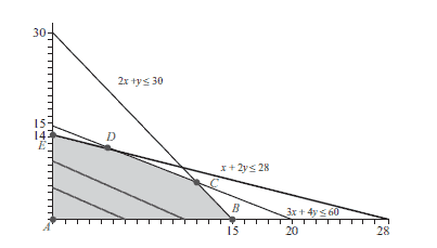
To illustrate this method, we continue with the example of Angie and Kiki’s lemonade stand. For convenience, we restate the problem here and reproduce the graph of the feasible region, along with some special points labeled and new lines in Figure $3.5$.
Let $x$ denote the number of glasses of sweet lemonade.
Let $y$ denote the number of glasses of tart lemonade.
We must
maximize: $R=1.25 x+1.5 y$
subject to:
$3 x+4 y \leq 60$ (lemons)
$x+2 y \leq 28$ (limes)
$116 \quad$ Graphical Linear Programming
Figure $3.5$ The feasible set for the lemonade stand problem.
$2 x+y \leq 30$ (tablespoons sugar)
$$
x \geq 0, y \geq 0
$$
Consider the feasible point $(6,0)$, where six glasses of sweet lemonade is made, but no tart lemonade is made. The revenue for that point is $R=1.25(6)+1.5(0)=\$ 7.50$. There are other feasible points that also produce a revenue of $\$ 7.50 ;$ for example, $(0,5)$ works. In fact, we claim that every feasible point on the line segment connecting $(6,0)$ to $(0,5)$ will produce the same revenue. Why is that? If we take our revenue function $R=1.25 x+$ to find all the points that generate the revenue of $\$ 7.50$, we obtain to find all the points that generate the revenue of $\$ 7.50$, we obtain $$ 1.25 x+1.5 y=7.50 \text {, } $$
Let’s find another level objective line – say, the one with revenue $\$ 15 .$ It is not hard to see that both $(12,0)$ and $(0,10)$ are on this line. The portion of this line that lies inside the feasible region is the second, longer line segment cutting across the feasible region in Figure $3.5$. It appears in the graph that the two level objective this second level objective line is
$1.25 x+1.5 y=15.00$.
In any line of the form $A x+B y=C$, the slope $m$ is determined by the coefficients $A$ and $B$; indeed, we have $m=-\frac{B}{A}$. Clearly, the various level objective lines differ only in the constant $C-$ they all have the same values of $A$ and $B$ (namely, $1.25$ and $1.5$, respectively). Thus, we see that all level objective lines have the same slope, so they are all parallel to each other. Furthermore, because the $A$ and $B$ in this problem are both positive (as they are in many problems in practice), larger and larger values of $x$ and $y$ lead to larger and larger values of $R$.
凸优化代考
我们现在讨论解决线性规划问题的技术。一般来说,涉及图形和图片的解决方法仅限于小问题。最著名的方法适用于只有两个决策变量的问题,但对约束的数量没有限制;换句话说,它适用于大小为 $m \times 2$ 的问题。在大多数文本中,这种方法被称为图形方法,但更准确的名称是决策空间中的绘图,因为坐标系的轴对应于两个决策变量。
还有另一种图形方法,我们称之为约束空间中的绘图。这种方法适用于大小为 $2\times n$ 的问题,因为坐标系的轴对应于两个约束,而决策变量的数量没有限制。在本节中,我们将介绍决策空间中的绘图,本章稍后将介绍约束空间中的绘图。实际问题是 $m \times 2$,是很容易从这种技术推导出线性规划的基本定理,也称为角点定理。
为了说明这种方法,我们继续以 Angie 和 Kiki 的柠檬水摊为例。为方便起见,我们在这里重述问题并重现可行区域的图形,以及图 $3.5$ 中标记的一些特殊点和新线。
令 $x$ 表示甜柠檬水的杯数。
令 $y$ 表示酸柠檬水的杯数。
我们必须
最大化:$R=1.25 x+1.5 y$
受制于:
$3 x+4 y \leq 60$(柠檬)
$x+2 y \leq 28$(酸橙)
$116 \quad$ 图形线性规划
图 $3.5$ 柠檬水摊问题的可行集。
$2 x+y \leq 30$(汤匙糖)
$$
x \geq 0, y \geq 0
$$
考虑可行点 $(6,0)$,其中制作了六杯甜柠檬水,但没有制作酸柠檬水。该点的收入为 $R=1.25(6)+1.5(0)=\$ 7.50$。还有其他可行的点也产生 $\$ 7.50 的收入;$ 例如,$(0,5)$ 有效。事实上,我们声称连接 $(6,0)$ 到 $(0,5)$ 的线段上的每个可行点都会产生相同的收入。这是为什么?如果我们用我们的收益函数 $R=1.25 x+$ 来找到所有产生 $\$ 7.50$ 收益的点,我们得到找到所有产生 $\$ 7.50$ 收益的点,我们得到 $$ 1.25 x+1.5 y=7.50 \text {, } $$
让我们找到另一个级别的目标线 – 比如说,收入 $\$ 15 .$ 不难看出 $(12,0)$ 和 $(0,10)$ 都在这条线上。这条线位于可行区域内的部分是第二条较长的线段,它在图 $3.5$ 中穿过可行区域。从图中可以看出,这个二级目标线的二级目标是
$1.25 x+1.5 y=15.00$。
在 $A x+B y=C$ 形式的任何直线中,斜率 $m$ 由系数 $A$ 和 $B$ 确定;事实上,我们有 $m=-\frac{B}{A}$。很明显,各层次目标线的区别仅在于常数$C-$,它们的$A$和$B$的值都相同(即分别为$1.25$和$1.5$)。因此,我们看到所有水平目标线具有相同的斜率,因此它们都相互平行。此外,由于该问题中的 $A$ 和 $B$ 都是正数(正如在实践中的许多问题中一样),$x$ 和 $y$ 的值越来越大导致 $R$ 的值越来越大.

数学代写| Chebyshev polynomials 数值分析代考 请认准UprivateTA™. UprivateTA™为您的留学生涯保驾护航。
时间序列分析代写
统计作业代写
随机过程代写
随机过程,是依赖于参数的一组随机变量的全体,参数通常是时间。 随机变量是随机现象的数量表现,其取值随着偶然因素的影响而改变。 例如,某商店在从时间t0到时间tK这段时间内接待顾客的人数,就是依赖于时间t的一组随机变量,即随机过程