数学代写|The Riemann zeta function 数论代考
数论代考
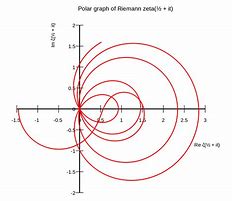
As recalled in Section $3.1$, the Riemann zeta function is defined first for complex numbers $s$ such that $\operatorname{Re}(s)>1$ by means of the absolutely convergent series
$$
\zeta(s)=\sum_{n \geqslant 1} \frac{1}{n^{s}} .
$$
By Lemma C.1.4, it has also the Euler product expansion
$$
\zeta(s)=\prod_{p}\left(1-p^{-s}\right)^{-1}
$$
in this region. Using this expression, we can compute the logarithmic derivative of the zeta function, always for $\operatorname{Re}(s)>1$. We obtain the Dirichlet series expansion (C.5)
$$
-\frac{\zeta^{\prime}}{\zeta}(s)=\sum_{p} \frac{(\log p) p^{-s}}{1-p^{-s}}=\sum_{n \geqslant 1} \frac{\Lambda(n)}{n^{s}}
$$
(using a geometric series expansion), where the function $\Lambda$ is called the von Mangoldt function, defined by
(C.6) $\Lambda(n)= \begin{cases}\log p & \text { if } n=p^{k} \text { for some prime } p \text { and some } k \geqslant 1 \ 0 & \text { otherwise. }\end{cases}$
In other words, up to the “thin” set of powers of primes with exponent $k \geqslant 2$, the function $\Lambda$ is the logarithm restricted to prime numbers.
Beyond the region of absolute convergence, it is known that the zeta function extends to a meromorphic function on all of $\mathbf{C}$, with a unique pole located at $s=1$, which is a simple pole with residue 1 (see the argument in Section $3.1$ for a simple proof of analytic continuation to $\operatorname{Re}(s)>0)$. More precisely, let
$$
\xi(s)=\pi^{-s / 2} \Gamma \mid\left(\frac{s}{2}\right) \zeta(s)
$$
for $\operatorname{Re}(s)>1$. Then $\xi$ extends to a meromorphic function on $\mathrm{C}$ with simple poles at $s=0$ and $s=1$, which satisfies the functional equation
$$
\xi(1-s)=\xi(s) .
$$
Because the Gamma function has poles at integers $-k$ for $k \geqslant 0$, it follows that $\zeta(-2 k)=0$ for $k \geqslant 1$ (the case $k=0$ is special because of the pole at $s=1$ ). The negative even integers are called the trivial zeros of $\zeta(s)$. Hadamard and de la Vallée Poussin proved (independently) that $\zeta(s) \neq 0$ for $\operatorname{Re}(s)=1$, and it follows that the non-trivial zeros of $\zeta(s)$ are located in the critical strip $0<\operatorname{Re}(s)<1$.
Proposition C.4.1. (1) For $1 / 2<\sigma<1$, we have
$$
\frac{1}{2 \mathrm{~T}} \int_{-\mathrm{T}}^{\mathrm{T}}|\zeta(\sigma+i t)|^{2} d t \longrightarrow \zeta(2 \sigma)
$$
as $\mathrm{T} \rightarrow+\infty$
174
(2) We have $\mathrm{T} \rightarrow+\infty$
See [117, Th. 7.2] for the proof of the first formula and [117, Th. 7.3] for the second (which is due to Hardy and Littlewood).
EXERCISE C.4.2. This exercise explains the proof of the first formula (which is easier than the second one).
(1) Prove that for $\frac{1}{2} \leqslant \sigma \leqslant \sigma^{\prime}<1$ and for $\mathrm{T} \geqslant 2$, we have
(Consider separately the sum where $m<\frac{1}{2} n$ and the remainder.)
(2) Prove that
$$
\frac{1}{2 \mathrm{~T}} \int_{-\mathrm{T}}^{\mathrm{T}}\left|\sum_{n \leqslant|t|} n^{-\sigma-i t}\right|^{2} d t \rightarrow \zeta(2 \sigma)
$$
as $\mathrm{T} \rightarrow+\infty$. (Expand the square and integrate using (1).)
(3) Conclude using Proposition C.4.5 below.
For much more information concerning the analytic properties of the Riemann zeta function, see [117]. Note however that the deeper arithmetic aspects are best understood in the larger framework of L-functions, from Dirichlet L-functions (which are discussed below in Section C.5) to automorphic L-functions (see, e.g, [59, Ch. 5]).
We will also use the Hadamard factorization of the Riemann zeta function. This is
如第 3.1 节所述,黎曼 zeta 函数首先定义为复数 $s$ 使得 $\operatorname{Re}(s)>1$ 通过绝对收敛级数
$$
\zeta(s)=\sum_{n \geqslant 1} \frac{1}{n^{s}} 。
$$
通过引理 C.1.4,它还具有欧拉乘积扩展
$$
\zeta(s)=\prod_{p}\left(1-p^{-s}\right)^{-1}
$$
在这个地区。使用这个表达式,我们可以计算 zeta 函数的对数导数,总是 $\operatorname{Re}(s)>1$。我们得到狄利克雷级数展开式(C.5)
$$
-\frac{\zeta^{\prime}}{\zeta}(s)=\sum_{p} \frac{(\log p) p^{-s}}{1-p^{-s}} =\sum_{n \geqslant 1} \frac{\Lambda(n)}{n^{s}}
$$
(使用几何级数展开),其中函数 $\Lambda$ 称为 von Mangoldt 函数,定义为
(C.6) $\Lambda(n)= \begin{cases}\log p & \text { if } n=p^{k} \text { 对于一些素数 } p \text { 和一些 } k \geqslant 1 \ 0 & \text { 否则。 }\结束{案例}$
换句话说,直到指数为$k \geqslant 2$ 的素数幂的“薄”集合,函数$\Lambda$ 是限制为素数的对数。
在绝对收敛区域之外,已知 zeta 函数扩展到所有 $\mathbf{C}$ 上的亚纯函数,其唯一极点位于 $s=1$,它是一个简单的极点,余数为 1 (参见第 3.1 节中的论点以获得对 $\operatorname{Re}(s)>0)$ 的分析延续的简单证明。更准确地说,让
$$
\xi(s)=\pi^{-s / 2} \Gamma \mid\left(\frac{s}{2}\right) \zeta(s)
$$
对于 $\operatorname{Re}(s)>1$。然后$\xi$ 扩展到$\mathrm{C}$ 上的亚纯函数,在$s=0$ 和$s=1$ 处有简单的极点,它满足泛函方程
$$
\xi(1-s)=\xi(s) 。
$$
因为对于 $k \geqslant 0$,Gamma 函数在整数 $-k$ 处有极点,因此对于 $k \geqslant 1$,$\zeta(-2 k)=0$($k=0$ 的情况是特别是因为 $s=1$ 处的极点)。负偶数称为 $\zeta(s)$ 的平凡零点。 Hadamard 和 de la Vallée Poussin(独立地)证明了对于 $\operatorname{Re}(s)=1$ 的 $\zeta(s)\neq 0$,因此 $\zeta(s )$ 位于关键带 $0<\operatorname{Re}(s)<1$ 中。
提案 C.4.1。 (1) 对于 $1 / 2<\sigma<1$,我们有
$$
\frac{1}{2 \mathrm{~T}} \int_{-\mathrm{T}}^{\mathrm{T}}|\zeta(\sigma+it)|^{2} dt \longrightarrow \泽塔(2 \sigma)
$$
作为 $\mathrm{T} \rightarrow+\infty$
174
(2) 我们有 $\mathrm{T} \rightarrow+\infty$
见 [117, Th. 7.2]为第一个公式的证明和[117,Th。 7.3] 第二个(这是由于哈代和利特尔伍德)。
练习 C.4.2。这个练习解释了第一个公式的证明(它比第二个更容易)。
(1) 证明对于 $\frac{1}{2} \leqslant \sigma \leqslant \sigma^{\prime}<1$ 和对于 $\mathrm{T} \geqslant 2$,我们有
(分别考虑 $m<\frac{1}{2} n$ 和余数的总和。)
(2) 证明
$$
\frac{1}{2 \mathrm{~T}} \int_{-\mathrm{T}}^{\mathrm{T}}\left|\sum_{n \leqslant|t|} n^{-\ sigma-i t}\right|^{2} dt \rightarrow \zeta(2 \sigma)
$$
如 $\mathrm{T} \rightarrow+\infty$。 (展开平方并使用 (1) 积分。)
(3) 使用下面的命题 C.4.5 结束。
有关黎曼 zeta 函数的分析性质的更多信息,请参见 [117]。然而请注意,更深层次的算术方面最好在更大的 L 函数框架中理解,从 Dirichlet L 函数(在下面的 C.5 节中讨论)到自守 L 函数(例如,参见 [59, Ch. 5])。
我们还将使用黎曼 zeta 函数的 Hadamard 因式分解。这是
数论代写
数论是纯粹数学的分支之一,主要研究整数的性质。整数可以是方程式的解(丢番图方程)。有些解析函数(像黎曼ζ函数)中包括了一些整数、质数的性质,透过这些函数也可以了解一些数论的问题。透过数论也可以建立实数和有理数之间的关系,并且用有理数来逼近实数(丢番图逼近)。
按研究方法来看,数论大致可分为初等数论和高等数论。初等数论是用初等方法研究的数论,它的研究方法本质上说,就是利用整数环的整除性质,主要包括整除理论、同余理论、连分数理论。高等数论则包括了更为深刻的数学研究工具。它大致包括代数数论、解析数论、计算数论等等。

其他相关科目课程代写:组合学Combinatorics集合论Set Theory概率论Probability组合生物学Combinatorial Biology组合化学Combinatorial Chemistry组合数据分析Combinatorial Data Analysis
my-assignmentexpert愿做同学们坚强的后盾,助同学们顺利完成学业,同学们如果在学业上遇到任何问题,请联系my-assignmentexpert™,我们随时为您服务!
在中世纪时,除了1175年至1200年住在北非和君士坦丁堡的斐波那契有关等差数列的研究外,西欧在数论上没有什么进展。
数论中期主要指15-16世纪到19世纪,是由费马、梅森、欧拉、高斯、勒让德、黎曼、希尔伯特等人发展的。最早的发展是在文艺复兴的末期,对于古希腊著作的重新研究。主要的成因是因为丢番图的《算术》(Arithmetica)一书的校正及翻译为拉丁文,早在1575年Xylander曾试图翻译,但不成功,后来才由Bachet在1621年翻译完成。
计量经济学代考
计量经济学是以一定的经济理论和统计资料为基础,运用数学、统计学方法与电脑技术,以建立经济计量模型为主要手段,定量分析研究具有随机性特性的经济变量关系的一门经济学学科。 主要内容包括理论计量经济学和应用经济计量学。 理论经济计量学主要研究如何运用、改造和发展数理统计的方法,使之成为经济关系测定的特殊方法。
相对论代考
相对论(英語:Theory of relativity)是关于时空和引力的理论,主要由愛因斯坦创立,依其研究对象的不同可分为狭义相对论和广义相对论。 相对论和量子力学的提出给物理学带来了革命性的变化,它们共同奠定了现代物理学的基础。
编码理论代写
编码理论(英语:Coding theory)是研究编码的性质以及它们在具体应用中的性能的理论。编码用于数据压缩、加密、纠错,最近也用于网络编码中。不同学科(如信息论、电机工程学、数学、语言学以及计算机科学)都研究编码是为了设计出高效、可靠的数据传输方法。这通常需要去除冗余并校正(或检测)数据传输中的错误。
编码共分四类:[1]
数据压缩和前向错误更正可以一起考虑。
复分析代考
学习易分析也已经很冬年了,七七八人的也续了圧少的书籍和论文。略作总结工作,方便后来人学 Đ参考。
复分析是一门历史悠久的学科,主要是研究解析函数,亚纯函数在复球面的性质。下面一昭这 些基本内容。
(1) 提到复变函数 ,首先需要了解复数的基本性左和四则运算规则。怎么样计算复数的平方根, 极坐标与 $x y$ 坐标的转换,复数的模之类的。这些在高中的时候囸本上都会学过。
(2) 复变函数自然是在复平面上来研究问题,此时数学分析里面的求导数之尖的运算就会很自然的 引入到复平面里面,从而引出解析函数的定义。那/研究解析函数的性贡就是关楗所在。最关键的 地方就是所谓的Cauchy一Riemann公式,这个是判断一个函数是否是解析函数的关键所在。
(3) 明白解析函数的定义以及性质之后,就会把数学分析里面的曲线积分 $a$ 的概念引入复分析中, 定义几乎是一致的。在引入了闭曲线和曲线积分之后,就会有出现复分析中的重要的定理: Cauchy 积分公式。 这个是易分析的第一个重要定理。