my-assignmentexpert™ Economics 经济学作业代写,免费提交作业要求, 满意后付款,成绩80\%以下全额退款,安全省心无顾虑。专业硕 博写手团队,所有订单可靠准时,保证 $100 \%$ 原创。my-assignmentexpert™, 最高质量的ECON经济学作业代写,服务覆盖北美、欧洲、澳洲等 国家。 在代写价格方面,考虑到同学们的经济条件,在保障代写质量的前提下,我们为客户提供最合理的价格。 由于economics作业种类很多,同时其中的大部分作业在字数上都没有具体要求,因此经济作业代写的价格不固定。通常在经济学专家查看完作业要求之后会给出报价。作业难度和截止日期对价格也有很大的影响。
想知道您作业确定的价格吗? 免费下单以相关学科的专家能了解具体的要求之后在1-3个小时就提出价格。专家的 报价比上列的价格能便宜好几倍。
my-assignmentexpert™ 为您的留学生涯保驾护航 在经济学作业代写方面已经树立了自己的口碑, 保证靠谱, 高质且原创的经济代写服务。我们的专家在经济学 代写方面经验极为丰富,各种economics相关的作业也就用不着 说。
我们提供的econ代写服务范围广, 其中包括但不限于:
- 微观经济学
- 货币银行学
- 数量经济学
- 宏观经济学
- 经济统计学
- 经济学理论
- 商务经济学
- 计量经济学
- 金融经济学
- 国际经济学
- 健康经济学
- 劳动经济学
Exchange Edgeworth box: prices and equilibria|Econ经济作业代写Economics代考
It is possible to add price information into Edgeworth boxes. If household $A$ buys a bundle $\left(x_{1}^{A}, x_{2}^{A}\right)$ with the same worth as his endowment, we have
$$
p_{1} x_{1}^{A}+p_{2} x_{2}^{A}=p_{1} \omega_{1}^{A}+p_{2} \omega_{2}^{A}
$$
Starting from an endowment point, positive prices $p_{1}$ and $p_{2}$ lead to negatively sloped budget lines for both individuals. In figure XIX.1, two price lines with prices $p_{1}^{l}<p_{1}^{h}$ are depicted. The indifference curves indicate which bundles the households prefer.
EXERCISE XIX.1. Why do the two price lines in figure XIX.1 cross at the endowment point w?
Of course, we would like to know whether these prices are compatible in the sense of allowing both agents to demand the preferred bundle. If that is the case, the prices and the bundles at these prices constitute a Walras equilibrium.
Definition of an exchange economy|ECON经济作业代写ECONOMICS代考
DEFINITION XIX.1 (EXCHANGE ECONOMY). An exchange economy is a tuple
$$
\mathcal{E}=\left(N, G,\left(\omega^{i}\right){i \in N},\left(\precsim^{i}\right){i \in N}\right)
$$
consisting of
- the set of agents $N={1,2, \ldots, n}$,
- the finite set of goods $G={1, \ldots, \ell}$,
and for every agent $i \in N$ - an endowment $\omega^{i}=\left(\omega_{1}^{i}, \ldots, \omega_{\ell}^{i}\right) \in \mathbb{R}_{+}^{\ell}$, and
- a preference relation $\precsim$.
Thus, every agent has property rights on endowments. The total endowment of an exchange economy is given by $\omega=\sum_{i \in N} \omega^{i}$. A household’s consumption possibilities are described by the budget. We refer the reader to chapter VI.
Excess Demand and Market Clearance|Econ经济作业代写Economics代考
Let us begin with the first case and consider player 1. The truthful announcement of his type leads to the provision of the public good and $z_{1}=0$. His utility is
$$
u_{1}(1,0, \ldots)=t_{1}-\frac{C}{n}
$$
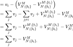
Player 1 has no incentive to overstate his willingness to pay (that will not change anything). Indeed, a utility change occurs only if player 1 understates his willingness to pay so that the public good is not provided. Then, player 1 has to pay $\sum_{j \in N \backslash{1}} m_{j}-\frac{n-1}{n} C$ (third case). Player 1 is harmed by this understatement:
$$
\begin{aligned}
u_{1}(1,0, \ldots) &=t_{1}-\frac{C}{n} \
& \geq\left(C-\sum_{j \in N \backslash{1}} m_{j}\right)-\frac{C}{n}(\text { case } 1) \
&=-\left(\sum_{j \in N \backslash{1}} m_{j}-\frac{n-1}{n} C\right) \
&=u_{1}\left(0, \sum_{j \in N \backslash{1}} m_{j}-\frac{n-1}{n} C, \ldots\right)
\end{aligned}
$$
Existence of the Walras equilibrium|ECON经济作业代写ECONOMICS代考
EXERCISE XIX.3. Consider a market where the excess demand of three individuals 1,2 , and 3 is given by
$$
z_{1}(p)=\frac{8}{p}-4, z_{2}(p)=\frac{4}{p}-2, z_{3}(p)=\frac{12}{p}-2 .
$$
Find the market-clearing price. Is individual 3 a buyer or a seller?
EXERCISE XIX.4. Abba (A) and Bertha (B) consider buying two goods 1 and 2, and face the price $p$ for good 1 in terms of good 2. Think of good 2 as the numéraire good with price 1 . Abba’s and Bertha’s utility functions $u_{A}$ and $u_{B}$, respectively, are given by $u_{A}\left(x_{1}^{A}, x_{2}^{A}\right)=\sqrt{x_{1}^{A}}+x_{2}^{A}$ and $u_{B}\left(x_{1}^{B}, x_{2}^{B}\right)=$ $\sqrt{x_{1}^{B}}+x_{2}^{B}$. Endowments are $\omega^{A}=(18,0)$ and $\omega^{B}=(0,10)$. Find the bundles demanded by these two agents. Then find the price $p$ that fulfills $\omega_{1}^{A}+\omega_{1}^{B}=x_{1}^{A}+x_{1}^{B}$ and $\omega_{2}^{A}+\omega_{2}^{B}=x_{2}^{A}+x_{2}^{B} .$
In the above exercise, what if only market 1 is cleared? The following lemma shows that local nonsatiation excludes this possibility.
Existence of the Nash equilibrium|ECON经济作业代写ECONOMICS代考
Example: The Cobb-Douglas exchange economy with two agents. We remember from chapter VI that income $m$ and Cobb-Douglas utility function
$$
u\left(x_{1}, x_{2}\right)=x_{1}^{a} x_{2}^{1-a}
$$
implies the household optimum
$$
\begin{aligned}
&x_{1}=a \frac{m}{p_{1}} \
&x_{2}=(1-a) \frac{m}{p_{2}} .
\end{aligned}
$$
Consider, now, individual 1 with Cobb-Douglas utility function $u^{1}$ and parameters $a_{1}($ for good 1$)$ and $1-a_{1}$ (for good 2). The initial endowment of individual 1 equals $\omega^{1}=(1,0)$. Individual 2 possesses a Cobb-Douglas utility function $u^{2}$ with parameters $a_{2}$ (for good 1$)$ and $1-a_{2}$ (for good 2). His initial endowment is $\omega^{2}=(0,1)$. Parameters $a_{1}$ and $a_{2}$ obey the following conditions: $0<a_{1}<1$ and $0<a_{2}<1$. Both goods are desired and the preferences obey local nonsatiation and weak monotonicity. According to lemma XIX.4, the market is in equilibrium only if it is cleared. Substituting the value of the endowment for income, we get individual 1’s demand for $\operatorname{good} 1$
Existence of the Walras equilibrium.|ECON经济作业代写ECONOMICS代考
2.5.3. Proof of the existence theorem XIX.1. In order to apply Brouwer’s fixed-point theorem to theorem XIX.1, we first construct a convex and compact set. The prices of the $\ell$ goods are normed such that the sum of the nonnegative (!, we have strict
monotonicity) prices equals 1. Just divide all prices by the sum of the prices. We can restrict our search for equilibrium prices to the $\ell-1$ – dimensional unit simplex:
$$
S^{\ell-1}=\left{p \in \mathbb{R}{+}^{\ell}: \sum{g=1}^{\ell} p_{g}=1\right}
$$
$S^{\ell-1}$ is nonempty, compact (closed and bounded as a subset of $\mathbb{R}^{\ell}$ ), and convex.
EXERCISE XIX.7. Draw $S^{1}=S^{2-1}$
The idea of the proof is as follows: First, we define a continuous function $f: S^{\ell-1} \rightarrow S^{\ell-1}$. Brouwer’s theorem
says that there is at least one fixed point of this function. Second, we show that such a fixed point fulfills the conditions of the Walras equilibrium.
The continuous function is defined by
$$
f=\left(\begin{array}{c}
f_{1} \
f_{2} \
\cdot \
\cdot \
\cdot \
f_{\ell}
\end{array}\right): S^{\ell-1} \rightarrow S^{\ell-1}
$$
and
$$
f_{g}(p)=\frac{p_{g}+\max \left(0, z_{g}(p)\right)}{1+\sum_{g^{\prime}=1}^{\ell} \max \left(0, z_{g^{\prime}}(p)\right)}, g=1, \ldots, \ell
$$
EXCHANGE EDGEWORTH BOX: PRICES AND EQUILIBRIA|ECON经济作业代写ECONOMICS代考
可以将价格信息添加到 Edgeworth 框中。如果家庭一种买一包(X1一种,X2一种)与他的禀赋一样,我们有
p1X1一种+p2X2一种=p1ω1一种+p2ω2一种
从禀赋点开始,价格为正p1和p2导致两个人的预算线呈负斜率。在图 XIX.1 中,两条价格线与价格p1一世<p1H被描绘。无差异曲线表明家庭更喜欢哪个捆绑包。
练习 XIX.1。为什么图 XIX.1 中的两条价格线在禀赋点 w 交叉?
当然,我们想知道这些价格在允许两个代理都要求首选捆绑包的意义上是否兼容。如果是这样,价格和这些价格的捆绑构成了瓦尔拉斯均衡。
DEFINITION OF AN EXCHANGE ECONOMY|ECON经济作业代写ECONOMICS代考
定义 XIX.1(交易所经济)。交换经济是一个元组
$$
\mathcal{E}=\left(N, G,\left(\omega^{i}\right) {i \in N},\left(\precsim^{i}\对) {i \in N}\right)
$$
由
- 代理集ñ=1,2,…,n,
- 有限的商品集G=1,…,ℓ,
并且对于每个代理一世∈ñ - 禀赋ω一世=(ω1一世,…,ωℓ一世)∈R+ℓ, 和
- 偏好关系≾.
因此,每个代理人对捐赠都有财产权。交换经济的总禀赋由下式给出ω=∑一世∈ñω一世. 家庭的消费可能性由预算描述。我们请读者参考第六章。
EXCESS DEMAND AND MARKET CLEARANCE|ECON经济作业代写ECONOMICS代考
让我们从第一个案例开始,考虑参与者 1。他类型的真实宣布导致提供公共物品和和1=0. 他的效用是
你1(1,0,…)=吨1−Cn
玩家 1 没有动机夸大他的支付意愿(这不会改变任何事情)。实际上,只有当参与者 1 低估了他的支付意愿以致没有提供公共物品时,效用才会发生变化。然后,玩家 1 必须支付∑j∈ñ∖1米j−n−1nC(第三种情况)。玩家 1 受到这种轻描淡写的伤害:
你1(1,0,…)=吨1−Cn ≥(C−∑j∈ñ∖1米j)−Cn( 案子 1) =−(∑j∈ñ∖1米j−n−1nC) =你1(0,∑j∈ñ∖1米j−n−1nC,…)
EXISTENCE OF THE WALRAS EQUILIBRIUM|ECON经济作业代写ECONOMICS代考
练习 XIX.3。考虑一个市场,其中三个人 1,2 和 3 的超额需求由下式给出
和1(p)=8p−4,和2(p)=4p−2,和3(p)=12p−2.
找到市场出清价。个人 3 是买家还是卖家?
练习 XIX.4。Abba (A) 和 Bertha (B) 考虑购买两种商品 1 和 2,并面对价格p就商品 2 而言,商品 1。将商品 2 视为价格为 1 的商品。Abba 和 Bertha 的效用函数你一种和你乙,分别由下式给出你一种(X1一种,X2一种)=X1一种+X2一种和你乙(X1乙,X2乙)= X1乙+X2乙. 禀赋是ω一种=(18,0)和ω乙=(0,10). 找到这两个代理要求的捆绑包。然后找到价格p满足ω1一种+ω1乙=X1一种+X1乙和ω2一种+ω2乙=X2一种+X2乙.
在上面的练习中,如果只有市场 1 被清算怎么办?以下引理表明局部不饱和排除了这种可能性。
EXISTENCE OF THE NASH EQUILIBRIUM|ECON经济作业代写ECONOMICS代考
示例:Cobb-Douglas 交换经济与两个代理人。我们记得在第六章中,收入米和 Cobb-Douglas 效用函数
你(X1,X2)=X1一种X21−一种
意味着家庭最优
X1=一种米p1 X2=(1−一种)米p2.
现在考虑具有 Cobb-Douglas 效用函数的个体 1你1和参数一种1(好 1)和1−一种1(对于好的 2)。个人1的初始禀赋等于ω1=(1,0). 个体 2 具有 Cobb-Douglas 效用函数你2带参数一种2(好 1)和1−一种2(对于好的 2)。他最初的禀赋是ω2=(0,1). 参数一种1和一种2遵守以下条件:0<一种1<1和0<一种2<1. 两种商品都是想要的,偏好服从局部不满足和弱单调性。根据引理 XIX.4,市场只有在出清时才处于均衡状态。用禀赋的价值代替收入,我们得到个人 1 的需求好的1
EXISTENCE OF THE WALRAS EQUILIBRIUM.|ECON经济作业代写ECONOMICS代考
2.5.3. 存在定理 XIX.1 的证明。为了将 Brouwer 不动点定理应用到定理 XIX.1,我们首先构造一个凸紧集。的价格ℓ商品经过规范,使得非负(!,我们有严格的单调性)价格之和等于 1。只需将所有价格除以价格之和即可。我们可以将我们对均衡价格的搜索限制在ℓ−1– 维数单位单纯形:
$$
S^{\ell-1}=\left{p \in \mathbb{R} {+}^{\ell}:\sum {g=1}^{\ell} p_{ g}=1\右}
$小号ℓ−1$一世sn○n和米p吨和,C○米p一种C吨(C一世○s和d一种ndb○你nd和d一种s一种s你bs和吨○F$Rℓ$),一种ndC○nv和X.和X和RC一世小号和X一世X.7.Dr一种在$小号1=小号2−1$吨H和一世d和一种○F吨H和pr○○F一世s一种sF○一世一世○在s:F一世rs吨,在和d和F一世n和一种C○n吨一世n你○你sF你nC吨一世○n$F:小号ℓ−1→小号ℓ−1$.乙r○你在和r′s吨H和○r和米s一种和s吨H一种吨吨H和r和一世s一种吨一世和一种s吨○n和F一世X和dp○一世n吨○F吨H一世sF你nC吨一世○n.小号和C○nd,在和sH○在吨H一种吨s你CH一种F一世X和dp○一世n吨F你一世F一世一世一世s吨H和C○nd一世吨一世○ns○F吨H和在一种一世r一种s和q你一世一世一世br一世你米.吨H和C○n吨一世n你○你sF你nC吨一世○n一世sd和F一世n和db和
f=\左(F1 F2 ⋅ ⋅ ⋅ Fℓ\right): S^{\ell-1} \rightarrow S^{\ell-1}
一种nd
f_{g}(p)=\frac{p_{g}+\max \left(0, z_{g}(p)\right)}{1+\sum_{g^{\prime}=1}^ {\ell} \max \left(0, z_{g^{\prime}}(p)\right)}, g=1, \ldots, \ell

matlab代写请认准UprivateTA™.
经济代写
计量经济学代写请认准my-assignmentexpert™ Economics 经济学作业代写
微观经济学代写请认准my-assignmentexpert™ Economics 经济学作业代写
宏观经济学代写请认准my-assignmentexpert™ Economics 经济学作业代写