
如果你也在 怎样代写实分析real analysis这个学科遇到相关的难题,请随时右上角联系我们的24/7代写客服。实分析real analysis是数学分析的一个分支,研究实数、实数序列和实数函数的行为。 实分析研究的实值序列和函数的一些特殊性质包括收敛性、极限、连续性、平稳性、可微分性和可整定性。实分析有别于复分析,后者涉及复数及其函数的研究。
实分析real analysis是数学中的一个经典分支,它的发展是为了使数和函数的研究正规化,并研究重要的概念,如极限和连续性。这些概念是微积分及其应用的基础。实物分析已经成为许多应用领域中不可或缺的工具。
实分析real analysis的基础知识:序列和数列的收敛性、连续性、可分性、黎曼积分、函数的序列和数列、均匀性以及极限操作的互换。
my-assignmentexpert™ 实分析real analysis作业代写,免费提交作业要求, 满意后付款,成绩80\%以下全额退款,安全省心无顾虑。专业硕 博写手团队,所有订单可靠准时,保证 100% 原创。my-assignmentexpert™, 最高质量的实分析real analysis作业代写,服务覆盖北美、欧洲、澳洲等 国家。 在代写价格方面,考虑到同学们的经济条件,在保障代写质量的前提下,我们为客户提供最合理的价格。 由于统计Statistics作业种类很多,同时其中的大部分作业在字数上都没有具体要求,因此复分析complex analysis作业代写的价格不固定。通常在经济学专家查看完作业要求之后会给出报价。作业难度和截止日期对价格也有很大的影响。
想知道您作业确定的价格吗? 免费下单以相关学科的专家能了解具体的要求之后在1-3个小时就提出价格。专家的 报价比上列的价格能便宜好几倍。
my-assignmentexpert™ 为您的留学生涯保驾护航 在数学mathematics作业代写方面已经树立了自己的口碑, 保证靠谱, 高质且原创的数学mathematics代写服务。我们的专家在实分析real analysis代写方面经验极为丰富,各种实分析real analysis相关的作业也就用不着 说。
我们提供的实分析real analysis及其相关学科的代写,服务范围广, 其中包括但不限于:
数学代写|实分析代写real analysis代考|The Inversion Formula
Our next goal is to prove the Inversion Formula for the Fourier transform. This theorem will show that if $f \in L^{1}(\mathbb{R})$ is such that its Fourier transform $\widehat{f}$ is also integrable, then we can recover $f$ from $\widehat{f}$. This is similar in spirit to Theorem 8.4.2, which states that the Fourier coefficients of a function $f \in L^{2}[0,1]$ can be used to recover $f$. That result follows from the fact that the trigonometric system $\left{e^{2 \pi i n x}\right}_{n \in \mathbb{Z}}$ is an orthonormal basis for $L^{2}[0,1]$. Here the situation is different, because the uncountable system $\left.\left{e^{2 \pi i \xi x}\right}\right}_{\xi \in \mathbb{R}}$ is not an orthonormal basis for $L^{2}(\mathbb{R})$. Indeed, $e^{2 \pi i \xi x}$ does not belong to $L^{2}(\mathbb{R})$ for any $\xi$. Even so, we will be able to use convolution and approximate identities to prove the Inversion Formula.
In order to state our results more succinctly, we introduce the following notation.
Definition 9.2.8 (Inverse Fourier Transform on $L^{1}(\mathbb{R})$ ). The inverse Fourier transform of $f \in L^{1}(\mathbb{R})$ is
$$
f(\xi)=\int_{-\infty}^{\infty} f(x) e^{2 \pi i \xi x} d x, \quad \text { for } \xi \in \mathbb{R} .
$$
The inverse Fourier transform behaves much like the Fourier transform. Indeed, if $f \in L^{1}(\mathbb{R})$ then both $\widehat{f}$ and $\hat{f}$ are well-defined continuous functions, and
$$
\stackrel{f}{f}(\xi)=\widehat{f}(-\xi), \quad \text { for all } \xi \in \mathbb{R} \text {. }
$$
Therefore, by making an appropriate change of variables, every result that we have stated so far for the Fourier transform has an analogue for the inverse Fourier transform.
The word “inverse” in Definition $9.2 .8$ needs to be interpreted with some care. Even if $f$ is integrable, its Fourier transform $g=\widehat{f}$ need not be integrable, and so its “inverse Fourier transform” $g$ might not even exist, much less equal $f$. However, we will prove in this section that if it is the case that $f$ and $\widehat{f}$ are both integrable then $(\widehat{f})^{\vee}=f$. It is only in this restricted sense that the inverse Fourier transform is the inverse of the Fourier transform for integrable functions. We state that theorem next, but then must develop some machinery before we can prove it.
数学代写|实分析代写REAL ANALYSIS代考|Smoothness and Decay
One of the important properties of the Fourier transform is that it interchanges smoothness and decay. For our first theorem in this direction, we will assume that $f \in L^{1}(\mathbb{R})$ has a certain amount of decay in the sense that $x^{m} f(x) \in L^{1}(\mathbb{R})$. This is not a pointwise decay requirement, but rather a kind of “average decay” assumption. As $x$ increases, the value of $\left|x^{m} f(x)\right|$ becomes increasingly large compared to the value of $|f(x)|$, yet if $x^{m} f(x)$ is integrable then the area under the graph of $\left|x^{m} f(x)\right|$, and not merely the area under $|f(x)|$, must be finite. We will prove that if $f$ satisfies this decay hypothesis, then $\widehat{f}$ is smooth in the sense that it is $m$-times differentiable. Although it is a slight abuse of notation, we will write $\left((-2 \pi i x)^{k} f(x)\right)^{\wedge}$ to denote the Fourier transform of the function $g(x)=(-2 \pi i x)^{k} f(x)$.
Theorem 9.2.13. Let $f \in L^{1}(\mathbb{R})$ and $m \in \mathbb{N}$ be given. Then
$$
x^{m} f(x) \in L^{1}(\mathbb{R}) \Longrightarrow \widehat{f} \in C_{0}^{m}(\mathbb{R})
$$
i.e., $\widehat{f}$ is m-times differentiable and $\widehat{f}, \widehat{f}^{\prime}, \ldots, \widehat{f}^{(m)} \in C_{0}(\mathbb{R})$. Furthermore, in this case we have $x^{k} f(x) \in L^{1}(\mathbb{R})$ for $k=0, \ldots, m$, and the $k$ th derivative of $\widehat{f}$ is the Fourier transform of $(-2 \pi i x)^{k} f(x)$ :
$$
\widehat{f}(k)=\frac{d^{k}}{d \xi^{k}} \widehat{f}=\left((-2 \pi i x)^{k} f(x)\right)^{\wedge}, \quad \text { for } k=0, \ldots, m
$$
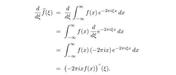
Proof. We will proceed by induction. The base step is $m=1$. To motivate equation (9.28) and its proof, note that if we were allowed to interchange a derivative with an integral, then we could write
$$
\begin{aligned}
\frac{d}{d \xi} \widehat{f}(\xi) &=\frac{d}{d \xi} \int_{-\infty}^{\infty} f(x) e^{-2 \pi i \xi x} d x \
&=\int_{-\infty}^{\infty} f(x) \frac{d}{d \xi} e^{-2 \pi i \xi x} d x \
&=\int_{-\infty}^{\infty} f(x)(-2 \pi i x) e^{-2 \pi i \xi x} d x \
&=(-2 \pi i x f(x))^{\wedge}(\xi) .
\end{aligned}
Essentially, our task is to justify this interchange.
实分析代写
数学代写|实分析代写REAL ANALYSIS代考|THE INVERSION FORMULA
我们的下一个目标是证明傅里叶变换的反演公式。这个定理将表明,如果F∈大号1(R)是这样的,它的傅里叶变换F^也是可积的,那么我们可以恢复F从F^. 这在精神上类似于定理 8.4.2,它指出函数的傅立叶系数F∈大号2[0,1]可以用来恢复F. 该结果源于以下事实:三角系统\left{e^{2 \pi i n x}\right}_{n \in \mathbb{Z}}\left{e^{2 \pi i n x}\right}_{n \in \mathbb{Z}}是一个正交基大号2[0,1]. 这里的情况不同,因为不可数系统\left.\left{e^{2 \pi i \xi x}\right}\right}_{\xi \in \mathbb{R}}\left.\left{e^{2 \pi i \xi x}\right}\right}_{\xi \in \mathbb{R}}不是标准正交基大号2(R). 确实,和2圆周率一世XX不属于大号2(R)对于任何X. 即便如此,我们将能够使用卷积和近似恒等式来证明反演公式。
为了更简洁地陈述我们的结果,我们引入以下符号。
定义 9.2.8(Inverse Fourier Transform on $L^{1}(\mathbb{R})$ ). The inverse Fourier transform of $f \in L^{1}(\mathbb{R})$ is
$$
f(\xi)=\int_{-\infty}^{\infty} f(x) e^{2 \pi i \xi x} d x, \quad \text { for } \xi \in \mathbb{R} .
$$
The inverse Fourier transform behaves much like the Fourier transform. Indeed, if $f \in L^{1}(\mathbb{R})$ then both $\widehat{f}$ and $\hat{f}$ are well-defined continuous functions, and
$$
\stackrel{f}{f}(\xi)=\widehat{f}(-\xi), \quad \text { for all } \xi \in \mathbb{R} \text {. }
$$
因此,通过对变量进行适当的更改,我们迄今为止为傅里叶变换陈述的每个结果都与傅里叶逆变换类似。
定义中的“逆”字9.2.8需要谨慎解释。即使F是可积的,它的傅里叶变换G=F^不必是可积的,因此它的“傅里叶逆变换”G甚至可能不存在,更不用说平等了F. 但是,我们将在本节中证明,如果是这样的话F和F^那么两者都是可积的(F^)∨=F. 仅在这种有限的意义上,傅里叶逆变换是可积函数的傅里叶变换的逆变换。我们接下来陈述这个定理,但在我们证明它之前必须开发一些机制。
数学代写|实分析代写REAL ANALYSIS代考|SMOOTHNESS AND DECAY
傅里叶变换的重要特性之一是它可以互换平滑度和衰减度。对于我们在这个方向上的第一个定理,我们将假设F∈大号1(R)有一定程度的衰变X米F(X)∈大号1(R). 这不是逐点衰减要求,而是一种“平均衰减”假设。作为X增加,的价值|X米F(X)|与价值相比变得越来越大|F(X)|, 但如果X米F(X)是可积的,那么图下的面积|X米F(X)|,而不仅仅是下面的区域|F(X)|, 必须是有限的。我们将证明如果F满足这个衰变假设,那么F^从某种意义上说是光滑的米-倍可微。虽然这是一个轻微的符号滥用,我们会写((−2圆周率一世X)到F(X))∧表示函数的傅里叶变换G(X)=(−2圆周率一世X)到F(X).
定理 9.2.13。让F∈大号1(R)和米∈ñ被给予。然后
X米F(X)∈大号1(R)⟹F^∈C0米(R)
IE,F^是 m 次可微的并且F^,F^′,…,F^(米)∈C0(R). 此外,在这种情况下,我们有X到F(X)∈大号1(R)为了到=0,…,米, 和到的导数F^是傅里叶变换(−2圆周率一世X)到F(X):
F^(到)=d到dX到F^=((−2圆周率一世X)到F(X))∧, 为了 到=0,…,米
证明。我们将通过归纳进行。基本步骤是米=1. 激发方程9.28及其证明,请注意,如果允许我们将导数与积分互换,那么我们可以写成
$$
ddXF^(X)=ddX∫−∞∞F(X)和−2圆周率一世XXdX =∫−∞∞F(X)ddX和−2圆周率一世XXdX =∫−∞∞F(X)(−2圆周率一世X)和−2圆周率一世XXdX =(−2圆周率一世XF(X))∧(X).
本质上,我们的任务是证明这种交换是合理的。

数学代写|实分析代写real analysis代考 请认准UprivateTA™. UprivateTA™为您的留学生涯保驾护航。
离散数学代写
Partial Differential Equations代写可以参考一份偏微分方程midterm答案解析