如果你也在 怎样代写数据可视化Intro to Data Analytics & Visualization这个学科遇到相关的难题,请随时右上角联系我们的24/7代写客服。数据可视化Intro to Data Analytics & Visualization数据可视化是以图画或图形的形式表示信息和数据(例如:图表、图形和地图)。数据可视化工具提供了一种方便的方式来查看和理解数据中的趋势、模式和异常值。数据可视化工具和技术对于分析海量信息和做出数据驱动的决策至关重要。使用图片来理解数据的概念自几个世纪以来一直被使用。数据可视化的一般类型是图表、表格、图形、地图、仪表盘。
数据可视化Intro to Data Analytics & Visualization析是分析数据集的过程,以便对他们所拥有的信息做出决策,越来越多地使用专门的软件和系统。数据分析技术被用于商业行业,使组织能够做出商业决策。数据可以帮助企业更好地了解他们的客户,改善他们的广告活动,个性化他们的内容,并提高他们的底线。数据分析的技术和过程已经被自动化为机械过程和算法,在原始数据上工作,供人使用。数据分析帮助企业优化其业绩。
my-assignmentexpert™ 数据可视化Intro to Data Analytics & Visualization作业代写,免费提交作业要求, 满意后付款,成绩80\%以下全额退款,安全省心无顾虑。专业硕 博写手团队,所有订单可靠准时,保证 100% 原创。my-assignmentexpert™, 最高质量的数据可视化Intro to Data Analytics & Visualization作业代写,服务覆盖北美、欧洲、澳洲等 国家。 在代写价格方面,考虑到同学们的经济条件,在保障代写质量的前提下,我们为客户提供最合理的价格。 由于统计Statistics作业种类很多,同时其中的大部分作业在字数上都没有具体要求,因此数据可视化Intro to Data Analytics & Visualization作业代写的价格不固定。通常在经济学专家查看完作业要求之后会给出报价。作业难度和截止日期对价格也有很大的影响。
想知道您作业确定的价格吗? 免费下单以相关学科的专家能了解具体的要求之后在1-3个小时就提出价格。专家的 报价比上列的价格能便宜好几倍。
my-assignmentexpert™ 为您的留学生涯保驾护航 在data analysis作业代写方面已经树立了自己的口碑, 保证靠谱, 高质且原创的data analysis代写服务。我们的专家在数据可视化Intro to Data Analytics & Visualization代写方面经验极为丰富,各种数据可视化Intro to Data Analytics & Visualization相关的作业也就用不着 说。
我们提供的数据可视化Intro to Data Analytics & Visualization及其相关学科的代写,服务范围广, 其中包括但不限于:

data analysis代写|数据可视化代写Intro to Data Analytics & Visualization代考|The inner working of agglomerative clustering
As briefly mentioned, agglomerative clustering refers to algorithms. Let’s start with the example of the data we used last in the previous chapter:
1 rownames (life.scaled) = life\$country
2 a=hclust (dist (life.scaled))
$3 \operatorname{par}(\mathrm{mf}$ row $=\mathrm{c}(1,2))$
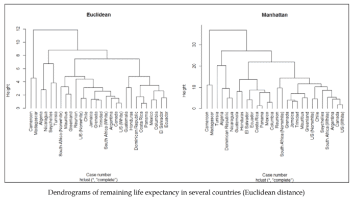
4 plot $(a$, hang $=-1, x l a b=$ “Case number”, main = “Euclidean”)
We started by adding the name of each country as the row name of the related case (line 1), in order to display it on the graph. The function hclust () was then used to generate a hierarchical agglomerative clustering solution from the data (line 2). The algorithm uses a distance matrix, provided as an argument (here the default is the Euclidean distance) to determine how to create a hierarchy of clusters. We have discussed measures of distance in the previous chapter. Please refer to this explanation if in doubt. Finally, the hclust object a at line 2 was plotted in a dendrogram (line 4 in the following diagram). At line 3 , we set the plotting area to include two plots.
The following figure (left panel), displays the clustering tree. At the beginning of the creation of the cluster hierarchy (or tree), each case is a cluster. Clusters are joined one by one on the basis of the distance between them (represented by the vertical lines); clusters with smaller distances are selected for merging. As can be seen from the distances plotted in the figure, holust () first joined Panama and Costa Rica in a new cluster. It then aggregated Canada and US (White) in a cluster, as they were the next cases with the smallest Euclidean distance, and it also did so for Grenada and Trinidad, Mexico and Columbia, and El Salvador and Ecuador. Next, it joined the cluster formed by Grenada and Trinidad with Jamaica. Clusters with the next smaller distance were then US (Nonwhite) and Chile, which were merged together. Then the cluster Canada and US (White) was merged with Argentina. The algorithm continued merging clusters until only one remained. It is quite interesting that hclust () produces life expectancy clusters that are closely related to the distance between countries; countries that are close geographically generally have similar life expectancies.
data analysis代写|数据可视化代写Intro to Data Analytics & Visualization代考|The use of hierarchical clustering on binary attributes
The previous datasets that we have used are composed of numerical attributes. Data is sometimes composed of binary attributes. By binary, we mean that there are only two possible modalities for the attribute. Examples of such attributes include characteristics such as gender (woman/man), currently married (yes/no), and organization type (private/public).
The distance metric to be provided to hclust () has to take the nature of the attributes into account; that is, it must be computed accordingly. The binary distance is the required type for such data. A distance matrix containing the binary distance can be obtained using the following line of code, where df is the data frame on which to compute the distance:
dist (df , method=”binary”)
Here we will use the Trucks dataset from the vcd package. Install and load it (as well as the data) using the following code:
install . packages (“vcd”)
install.pack library (vcd) data (Trucks) head (Trucks)
DATA ANALYSIS代写|数据可视化代写INTRO TO DATA ANALYTICS & VISUALIZATION代考|Exploring the results of votes in Switzerland
In this section, we will examine the case of another dataset. This dataset represents the percentage of acceptance of the themes of federal (national) voting objects in Switzerland in 2001 . The first rows of data are in the following table. The rows represent the cantons (the Swiss name for states). The columns (except the first) represent the topic of the voting. The values are the percentage of acceptance of the topic of voting. The data has been retrieved from the Swiss Statistics Office (www.bfs . admin.ch) and are provided in the folder for this chapter (file swiss_votes. dat).
To load the data, save the file in your working directory or change the working directory (use setwd () to the path of the file) and type the following line of code. Here, the sep argument is set to indicate that tabulations are used as separators, and the header argument is set to $\mathrm{T}$ (true), meaning that the provided data has column headers (attribute names):
swiss_votes $=$ read.table (“swiss_votes.dat”, sep $=” \backslash t^{\prime \prime}$,
header = $\mathrm{T}$ )
数据可视化代写
DATA ANALYSIS代写|数据可视化代写INTRO TO DATA ANALYTICS & VISUALIZATION代考|THE INNER WORKING OF AGGLOMERATIVE CLUSTERING
如前所述,凝聚聚类是指算法。让我们从上一章最后使用的数据示例开始:
1 rownamesl一世F和.sC一种l和d= 生活$国家
2 a=hclustd一世s吨(l一世F和.sC一种l和d)
3关于(米F排=C(1,2))
4地块(一种, 悬挂=−1,Xl一种b=“Case number”, main = “Euclidean”)
我们首先将每个国家的名称添加为相关案例的行名l一世n和1,以便在图表上显示它。函数 hclust然后用于从数据生成层次凝聚聚类解决方案l一世n和2. 该算法使用距离矩阵,作为参数提供H和r和吨H和d和F一种在l吨一世s吨H和和在Cl一世d和一种nd一世s吨一种nC和以确定如何创建集群的层次结构。我们在前一章讨论了距离的度量。如有疑问,请参阅此说明。最后,将第 2 行的 hclust 对象 a 绘制在树状图中l一世n和4一世n吨H和F这ll这在一世nGd一世一种Gr一种米. 在第 3 行,我们将绘图区域设置为包括两个绘图。
下图l和F吨p一种n和l, 显示聚类树。在开始创建集群层次结构时这r吨r和和,每个案例都是一个集群。集群根据它们之间的距离一一连接r和pr和s和n吨和db是吨H和在和r吨一世C一种ll一世n和s; 选择距离较小的簇进行合并。从图中绘制的距离可以看出,holust首先加入巴拿马和哥斯达黎加的新集群。然后它聚合了加拿大和美国在H一世吨和在一个集群中,因为它们是欧几里得距离最小的下一个案例,格林纳达和特立尼达、墨西哥和哥伦比亚、萨尔瓦多和厄瓜多尔也是如此。接下来,它加入了由格林纳达和特立尼达与牙买加组成的集群。距离下一个更小的集群是美国ñ这n在H一世吨和和智利合并在一起。然后集群加拿大和美国在H一世吨和并入阿根廷。该算法继续合并集群,直到只剩下一个。很有趣的是 hclust产生与国家间距离密切相关的预期寿命集群;地理位置相近的国家通常具有相似的预期寿命。
DATA ANALYSIS代写|数据可视化代写INTRO TO DATA ANALYTICS & VISUALIZATION代考|THE USE OF HIERARCHICAL CLUSTERING ON BINARY ATTRIBUTES
我们之前使用的数据集是由数字属性组成的。数据有时由二进制属性组成。通过二进制,我们的意思是该属性只有两种可能的模态。此类属性的示例包括性别等特征在这米一种n/米一种n, 目前已婚是和s/n这, 和组织类型pr一世在一种吨和/p在bl一世C.
要提供给 hclust 的距离度量必须考虑属性的性质;也就是说,它必须相应地计算。二进制距离是此类数据所需的类型。可以使用以下代码行获得包含二进制距离的距离矩阵,其中 df 是用于计算距离的数据帧:
distdF,米和吨H这d=”b一世n一种r是”
在这里,我们将使用 vcd 包中的卡车数据集。安装并加载它一种s在和ll一种s吨H和d一种吨一种使用以下代码:
安装。包“在Cd”
install.pack 库在Cd数据吨r在Cķs头吨r在Cķs
DATA ANALYSIS代写|数据可视化代写INTRO TO DATA ANALYTICS & VISUALIZATION代考|EXPLORING THE RESULTS OF VOTES IN SWITZERLAND
在本节中,我们将研究另一个数据集的情况。该数据集代表接受联邦主题的百分比n一种吨一世这n一种l2001年瑞士的投票对象。第一行数据如下表所示。行代表州吨H和小号在一世ssn一种米和F这rs吨一种吨和s. 列和XC和p吨吨H和F一世rs吨代表投票的主题。这些值是接受投票主题的百分比。数据取自瑞士统计局在在在.bFs.一种d米一世n.CH并在本章的文件夹中提供F一世l和s在一世ss在这吨和s.d一种吨.
要加载数据,请将文件保存在工作目录中或更改工作目录在s和s和吨在d(到文件的路径)并键入以下代码行。这里,sep 参数设置为表示使用制表符作为分隔符,header 参数设置为吨 吨r在和,这意味着提供的数据具有列标题一种吨吨r一世b在吨和n一种米和s:
瑞士投票=读表“s在一世ss在这吨和s.d一种吨”,s和p$=”∖吨′′$,H和一种d和r=$吨$

data analysis代写|数据可视化代写Intro to Data Analytics & Visualization代考 请认准UprivateTA™. UprivateTA™为您的留学生涯保驾护航。
电磁学代考
物理代考服务:
物理Physics考试代考、留学生物理online exam代考、电磁学代考、热力学代考、相对论代考、电动力学代考、电磁学代考、分析力学代考、澳洲物理代考、北美物理考试代考、美国留学生物理final exam代考、加拿大物理midterm代考、澳洲物理online exam代考、英国物理online quiz代考等。
光学代考
光学(Optics),是物理学的分支,主要是研究光的现象、性质与应用,包括光与物质之间的相互作用、光学仪器的制作。光学通常研究红外线、紫外线及可见光的物理行为。因为光是电磁波,其它形式的电磁辐射,例如X射线、微波、电磁辐射及无线电波等等也具有类似光的特性。
大多数常见的光学现象都可以用经典电动力学理论来说明。但是,通常这全套理论很难实际应用,必需先假定简单模型。几何光学的模型最为容易使用。
相对论代考
上至高压线,下至发电机,只要用到电的地方就有相对论效应存在!相对论是关于时空和引力的理论,主要由爱因斯坦创立,相对论的提出给物理学带来了革命性的变化,被誉为现代物理性最伟大的基础理论。
流体力学代考
流体力学是力学的一个分支。 主要研究在各种力的作用下流体本身的状态,以及流体和固体壁面、流体和流体之间、流体与其他运动形态之间的相互作用的力学分支。
随机过程代写
随机过程,是依赖于参数的一组随机变量的全体,参数通常是时间。 随机变量是随机现象的数量表现,其取值随着偶然因素的影响而改变。 例如,某商店在从时间t0到时间tK这段时间内接待顾客的人数,就是依赖于时间t的一组随机变量,即随机过程
Matlab代写
MATLAB 是一种用于技术计算的高性能语言。它将计算、可视化和编程集成在一个易于使用的环境中,其中问题和解决方案以熟悉的数学符号表示。典型用途包括:数学和计算算法开发建模、仿真和原型制作数据分析、探索和可视化科学和工程图形应用程序开发,包括图形用户界面构建MATLAB 是一个交互式系统,其基本数据元素是一个不需要维度的数组。这使您可以解决许多技术计算问题,尤其是那些具有矩阵和向量公式的问题,而只需用 C 或 Fortran 等标量非交互式语言编写程序所需的时间的一小部分。MATLAB 名称代表矩阵实验室。MATLAB 最初的编写目的是提供对由 LINPACK 和 EISPACK 项目开发的矩阵软件的轻松访问,这两个项目共同代表了矩阵计算软件的最新技术。MATLAB 经过多年的发展,得到了许多用户的投入。在大学环境中,它是数学、工程和科学入门和高级课程的标准教学工具。在工业领域,MATLAB 是高效研究、开发和分析的首选工具。MATLAB 具有一系列称为工具箱的特定于应用程序的解决方案。对于大多数 MATLAB 用户来说非常重要,工具箱允许您学习和应用专业技术。工具箱是 MATLAB 函数(M 文件)的综合集合,可扩展 MATLAB 环境以解决特定类别的问题。可用工具箱的领域包括信号处理、控制系统、神经网络、模糊逻辑、小波、仿真等。