
如果你也在 怎样代写matlab这个学科遇到相关的难题,请随时右上角联系我们的24/7代写客服。matlab是由数学家和计算机程序员Cleve Moler发明的。MATLAB的想法是基于他1960年代的博士论文。Moler成为新墨西哥大学的一名数学教授,并开始为他的学生开发MATLAB 作为一种爱好。他在1967年与他曾经的论文导师George Forsythe开发了MATLAB的初始线性代数编程。随后在1971年为线性方程编写Fortran代码。
matlab的第一个早期版本是在20世纪70年代末完成的。1979年2月,该软件在加利福尼亚州的海军研究生院首次向公众披露。 MATLAB的早期版本是简单的矩阵计算器,有71个预置函数。当时,MATLAB被免费分发到各大学。Moler会在他访问的大学留下拷贝,该软件在大学校园的数学系中培养了一批强大的追随者。
my-assignmentexpert™ matlab作业代写,免费提交作业要求, 满意后付款,成绩80\%以下全额退款,安全省心无顾虑。专业硕 博写手团队,所有订单可靠准时,保证 100% 原创。my-assignmentexpert™, 最高质量的matlab作业代写,服务覆盖北美、欧洲、澳洲等 国家。 在代写价格方面,考虑到同学们的经济条件,在保障代写质量的前提下,我们为客户提供最合理的价格。 由于统计Statistics作业种类很多,同时其中的大部分作业在字数上都没有具体要求,因此matlab作业代写的价格不固定。通常在经济学专家查看完作业要求之后会给出报价。作业难度和截止日期对价格也有很大的影响。
想知道您作业确定的价格吗? 免费下单以相关学科的专家能了解具体的要求之后在1-3个小时就提出价格。专家的 报价比上列的价格能便宜好几倍。
my-assignmentexpert™ 为您的留学生涯保驾护航 在数学Mathematics作业代写方面已经树立了自己的口碑, 保证靠谱, 高质且原创的数学Mathematics代写服务。我们的专家在matlab代写方面经验极为丰富,各种matlab相关的作业也就用不着 说。
我们提供的matlab及其相关学科的代写,服务范围广, 其中包括但不限于:
数学代写|matlab代写|Introduction
Ordinary differential equations (ODEs) are used throughout engineering, mathematics, and science to describe how physical quantities change, so an introductory course on elementary ODEs and their solutions is a standard part of the curriculum in these fields. Such a course provides insight, but the solution techniques discussed are generally unable to deal with the large, complicated, and nonlinear systems of equations seen in practice. This book is about solving ODEs numerically. Each of the authors has decades of experience in both industry and academia helping people like yourself solve problems. We begin in this chapter with a discussion of what is meant by a numerical solution with standard methods and, in particular, of what you can reasonably expect of standard software. In the chapters that follow, we discuss briefly the most popular methods for important classes of ODE problems. Examples are used throughout to show how to solve realistic problems. MatLAB (2000) is used to solve nearly all these problems because it is a very convenient and widely used problem-solving environment (PSE) with quality solvers that are exceptionally easy to use. It is also such a high-level programming language that programs are short, making it practical to list complete programs for all the examples. We also include some discussion of software available in other computing environments. Indeed, each of the authors has written ODE solvers widely used in general scientific computing.
An ODE represents a relationship between a function and its derivatives. One such relation taken up early in calculus courses is the linear ordinary differential equation
$$
y^{\prime}(t)=y(t)
$$
which is to hold for, say, $0 \leq t \leq 10$. As we learn in a first course, we need more than just an ODE to specify a solution. Often solutions are specified by means of an initial value. For example, there is a unique solution of the ODE (1.1) for which $y(0)=1$, namely $y(t)=e^{t}$. This is an example of an initial value problem (IVP) for an ODE. Like this example, the IVPs that arise in practice generally have one and only one solution. Sometimes solutions are specified in a more complicated way. This is important in practice, but it is not often discussed in a first course except possibly for the special case of Sturm-Liouville eigenproblems. Suppose that $y(x)$ satisfies the equation
$$
y^{\prime \prime}(x)+y(x)=0
$$
for $0 \leq x \leq b$. When a solution of this ODE is specified by conditions at both ends of the interval such as
$$
y(0)=0, \quad y(b)=0
$$
数学代写|matlab代写|Existence, Uniqueness, and Well-Posedness
From the title of this section you might imagine that this is just another example of mathematicians being fussy. But it is not: it is about whether you will be able to solve a problem at all and, if you can, how well. In this book we’ll see a good many examples of physical problems that do not have solutions for certain values of parameters. We’ll also see physical problems that have more than one solution. Clearly we’ll have trouble computing a solution that does not exist, and if there is more than one solution then we’ll have trouble computing the “right” one. Although there are mathematical results that guarantee a problem has a solution and only one, there is no substitute for an understanding of the phenomena being modeled.
Existence and uniqueness are much simpler for IVPs than BVPs, and the class of DDEs we consider can be understood in terms of IVPs, so we concentrate here on IVPs and defer to later chapters a fuller discussion of BVPs and DDEs. The vast majority of IVPs that arise in practice can be written as a system of $d$ explicit first-order ODEs:
$$
\begin{aligned}
y_{1}^{\prime}(t) &=f_{1}\left(t, y_{1}(t), y_{2}(t), \ldots, y_{d}(t)\right) \
y_{2}^{\prime}(t) &=f_{2}\left(t, y_{1}(t), y_{2}(t), \ldots, y_{d}(t)\right) \
& \vdots \
y_{d}^{\prime}(t) &=f_{n}\left(t, y_{1}(t), y_{2}(t), \ldots, y_{d}(t)\right)
\end{aligned}
$$
For brevity we generally write this system in terms of the (column) vectors
$$
y(t)=\left(\begin{array}{c}
y_{1}(t) \
y_{2}(t) \
\vdots \
y_{d}(t)
\end{array}\right), \quad f(t, y(t))=\left(\begin{array}{c}
f_{1}(t, y(t)) \
f_{2}(t, y(t)) \
\vdots \
f_{d}(t, y(t))
\end{array}\right)
$$
as
$$
y^{\prime}(t)=f(t, y(t))
$$
数学代写|matlab代写|Standard Form
Ordinary differential equations arise in the most diverse forms. In order to solve an ODE problem, you must first write it in a form acceptable to your code. By far the most common form accepted by IVP solvers is the system of first-order equations discussed in Section 1.2,
$$
y^{\prime}=f(t, y)
$$
The MatLAB IVP solvers accept ODEs of the more general form
$$
M(t, y) y^{\prime}=F(t, y)
$$
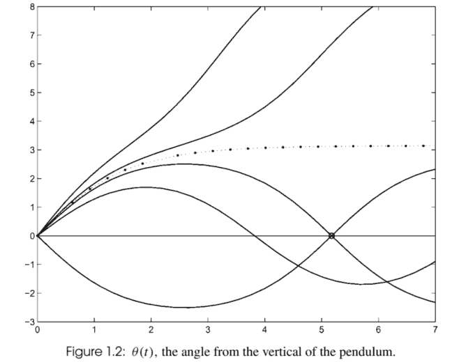
involving a nonsingular mass matrix $M(t, y)$. These equations can be written in the form (1.15) with $f(t, y)=M(t, y)^{-1} F(t, y)$, but for some kinds of problems the form (1.16) is more convenient and more efficient. With either form, we must formulate the ODEs as a system of first-order equations. The usual way to do this is to introduce new dependent variables. You must introduce a new variable for each of the dependent variables in the original form of the problem. In addition, a new variable is needed for each derivative of an original variable up to one less than the highest derivative appearing in the original equations. For each new variable, you need an equation for its first derivative expressed in terms of the new variables. A little manipulation using the definitions of the new variables and the original equations is then required to write the new equations in the form (1.15) (or (1.16)). This is harder to explain in words than it is to do, so let’s look at some examples. To put the ODE (1.6) describing the motion of a pendulum in standard form, we begin with a new variable $y_{1}(t)=\theta(t)$. The second derivative of $\theta(t)$ appears in the equation, so we need to introduce one more new variable, $y_{2}(t)=\theta^{\prime}(t)$. For these variables we have
$$
\begin{aligned}
&y_{1}^{\prime}(t)=\theta^{\prime}(t)=y_{2}(t) \
&y_{2}^{\prime}(t)=\theta^{\prime \prime}(t)=-\sin (\theta(t))=-\sin \left(y_{1}(t)\right)
\end{aligned}
$$
matlab代做
数学代写|MATLAB代写|INTRODUCTION
常微分方程这D和s在整个工程、数学和科学中用于描述物理量如何变化,因此关于基本 ODE 及其解决方案的介绍性课程是这些领域课程的标准部分。这样的课程提供了洞察力,但所讨论的求解技术通常无法处理在实践中看到的大型、复杂和非线性方程组。这本书是关于数值求解 ODE 的。每位作者都有数十年的工业和学术界经验,帮助像你这样的人解决问题。我们在本章开始讨论使用标准方法的数值解的含义,特别是您可以合理地期望标准软件的含义。在接下来的章节中,我们简要讨论重要类别的 ODE 问题最流行的方法。示例贯穿始终以展示如何解决实际问题。MatLAB2000用于解决几乎所有这些问题,因为它是一个非常方便且广泛使用的问题解决环境磷小号和具有非常易于使用的高质量求解器。它也是一种高级编程语言,程序很短,因此可以为所有示例列出完整的程序。我们还讨论了其他计算环境中可用的软件。事实上,每位作者都编写了广泛用于一般科学计算的 ODE 求解器。
ODE 表示函数与其导数之间的关系。微积分课程早期采用的一种这样的关系是线性常微分方程
是′(吨)=是(吨)
也就是说,坚持,说,0≤吨≤10. 正如我们在第一门课程中学习的那样,我们需要的不仅仅是一个 ODE 来指定一个解决方案。通常解决方案是通过初始值指定的。例如,存在 ODE 的唯一解1.1为此是(0)=1,即是(吨)=和吨. 这是一个初始值问题的例子一世在磷对于 ODE。像这个例子一样,实践中出现的IVP通常只有一个解决方案。有时以更复杂的方式指定解决方案。这在实践中很重要,但在第一门课程中通常不会讨论,除非可能是 Sturm-Liouville 特征问题的特殊情况。假设是(X)满足方程
是′′(X)+是(X)=0
为了0≤X≤b. 当此 ODE 的解由区间两端的条件指定时,例如
是(0)=0,是(b)=0
数学代写|MATLAB代写|EXISTENCE, UNIQUENESS, AND WELL-POSEDNESS
从本节的标题中,您可能会认为这只是数学家挑剔的另一个例子。但事实并非如此:它是关于你是否能够解决一个问题,如果可以的话,解决的程度如何。在本书中,我们将看到很多物理问题的例子,这些例子对某些参数值没有解决方案。我们还将看到有不止一种解决方案的物理问题。显然,我们将难以计算一个不存在的解决方案,如果有多个解决方案,那么我们将难以计算“正确”的一个。尽管有数学结果可以保证一个问题有一个解决方案并且只有一个,但没有什么可以替代对所建模现象的理解。
IVP 的存在性和唯一性比 BVP 简单得多,而且我们考虑的 DDE 类可以根据 IVP 来理解,因此我们在此集中讨论 IVP,并在后面的章节中更全面地讨论 BVP 和 DDE。实践中出现的绝大多数 IVP 都可以写成一个系统d显式一阶 ODE:
是1′(吨)=F1(吨,是1(吨),是2(吨),…,是d(吨)) 是2′(吨)=F2(吨,是1(吨),是2(吨),…,是d(吨)) ⋮ 是d′(吨)=Fn(吨,是1(吨),是2(吨),…,是d(吨))
为简洁起见,我们通常根据C这l在米n矢量图
$$
y(t)=\left(\begin{array}{c}
y_{1}(t) \
y_{2}(t) \
\vdots \
y_{d}(t)
\end{array}\right), \quad f(t, y(t))=\left(\begin{array}{c}
f_{1}(t, y(t)) \
f_{2}(t, y(t)) \
\vdots \
f_{d}(t, y(t))
\end{array}\right)
$$
as
$$
y^{\prime}(t)=f(t, y(t))
$$
数学代写|MATLAB代写|STANDARD FORM
常微分方程以最多样化的形式出现。为了解决 ODE 问题,您必须首先以您的代码可接受的形式编写它。到目前为止,IVP 求解器接受的最常见形式是第 1.2 节中讨论的一阶方程组,
是′=F(吨,是)
MatLAB IVP 求解器接受更一般形式的 ODE
米(吨,是)是′=F(吨,是)
涉及非奇异质量矩阵米(吨,是). 这些方程可以写成以下形式1.15和F(吨,是)=米(吨,是)−1F(吨,是),但对于某些类型的问题,形式1.16更方便,更高效。无论采用哪种形式,我们都必须将 ODE 表示为一阶方程组。通常的方法是引入新的因变量。您必须为问题的原始形式中的每个因变量引入一个新变量。此外,对于原始变量的每个导数,都需要一个新变量,最多比原始方程中出现的最高导数小一。对于每个新变量,您需要一个方程来表示它的一阶导数,用新变量表示。然后需要使用新变量和原始方程的定义进行一些操作,以将新方程写成以下形式1.15 这r(1.16)。这很难用语言来解释,所以让我们看一些例子。把 ODE1.6以标准形式描述摆的运动,我们从一个新变量开始是1(吨)=θ(吨). 的二阶导数θ(吨)出现在方程中,所以我们需要再引入一个新变量,是2(吨)=θ′(吨). 对于这些变量,我们有
$$
\begin{aligned}
&y_{1}^{\prime}(t)=\theta^{\prime}(t)=y_{2}(t) \
&y_{2}^{\prime}(t)=\theta^{\prime \prime}(t)=-\sin (\theta(t))=-\sin \left(y_{1}(t)\right)
\end{aligned}
$$

数学代写|matlab代写 请认准UprivateTA™. UprivateTA™为您的留学生涯保驾护航。
微观经济学代写
微观经济学是主流经济学的一个分支,研究个人和企业在做出有关稀缺资源分配的决策时的行为以及这些个人和企业之间的相互作用。my-assignmentexpert™ 为您的留学生涯保驾护航 在数学Mathematics作业代写方面已经树立了自己的口碑, 保证靠谱, 高质且原创的数学Mathematics代写服务。我们的专家在图论代写Graph Theory代写方面经验极为丰富,各种图论代写Graph Theory相关的作业也就用不着 说。
线性代数代写
线性代数是数学的一个分支,涉及线性方程,如:线性图,如:以及它们在向量空间和通过矩阵的表示。线性代数是几乎所有数学领域的核心。
博弈论代写
现代博弈论始于约翰-冯-诺伊曼(John von Neumann)提出的两人零和博弈中的混合策略均衡的观点及其证明。冯-诺依曼的原始证明使用了关于连续映射到紧凑凸集的布劳威尔定点定理,这成为博弈论和数学经济学的标准方法。在他的论文之后,1944年,他与奥斯卡-莫根斯特恩(Oskar Morgenstern)共同撰写了《游戏和经济行为理论》一书,该书考虑了几个参与者的合作游戏。这本书的第二版提供了预期效用的公理理论,使数理统计学家和经济学家能够处理不确定性下的决策。
微积分代写
微积分,最初被称为无穷小微积分或 “无穷小的微积分”,是对连续变化的数学研究,就像几何学是对形状的研究,而代数是对算术运算的概括研究一样。
它有两个主要分支,微分和积分;微分涉及瞬时变化率和曲线的斜率,而积分涉及数量的累积,以及曲线下或曲线之间的面积。这两个分支通过微积分的基本定理相互联系,它们利用了无限序列和无限级数收敛到一个明确定义的极限的基本概念 。
计量经济学代写
什么是计量经济学?
计量经济学是统计学和数学模型的定量应用,使用数据来发展理论或测试经济学中的现有假设,并根据历史数据预测未来趋势。它对现实世界的数据进行统计试验,然后将结果与被测试的理论进行比较和对比。
根据你是对测试现有理论感兴趣,还是对利用现有数据在这些观察的基础上提出新的假设感兴趣,计量经济学可以细分为两大类:理论和应用。那些经常从事这种实践的人通常被称为计量经济学家。
Matlab代写
MATLAB 是一种用于技术计算的高性能语言。它将计算、可视化和编程集成在一个易于使用的环境中,其中问题和解决方案以熟悉的数学符号表示。典型用途包括:数学和计算算法开发建模、仿真和原型制作数据分析、探索和可视化科学和工程图形应用程序开发,包括图形用户界面构建MATLAB 是一个交互式系统,其基本数据元素是一个不需要维度的数组。这使您可以解决许多技术计算问题,尤其是那些具有矩阵和向量公式的问题,而只需用 C 或 Fortran 等标量非交互式语言编写程序所需的时间的一小部分。MATLAB 名称代表矩阵实验室。MATLAB 最初的编写目的是提供对由 LINPACK 和 EISPACK 项目开发的矩阵软件的轻松访问,这两个项目共同代表了矩阵计算软件的最新技术。MATLAB 经过多年的发展,得到了许多用户的投入。在大学环境中,它是数学、工程和科学入门和高级课程的标准教学工具。在工业领域,MATLAB 是高效研究、开发和分析的首选工具。MATLAB 具有一系列称为工具箱的特定于应用程序的解决方案。对于大多数 MATLAB 用户来说非常重要,工具箱允许您学习和应用专业技术。工具箱是 MATLAB 函数(M 文件)的综合集合,可扩展 MATLAB 环境以解决特定类别的问题。可用工具箱的领域包括信号处理、控制系统、神经网络、模糊逻辑、小波、仿真等。