
如果你也在 怎样代写网络分析Network Analysis SCTE2022这个学科遇到相关的难题,请随时右上角联系我们的24/7代写客服。网络分析Network Analysis是一套综合技术,用于描述行为者之间的关系,并分析从这些关系的重复出现中产生的社会结构。其基本假设是,通过分析实体之间的关系,可以对社会现象做出更好的解释。这种分析是通过收集以矩阵形式组织的关系数据进行的。如果行动者被描述为节点,而他们的关系被描述为节点对之间的线,那么社会网络的概念就从一个隐喻变成了一个可操作的分析工具,它利用了图论和矩阵及关系代数的数学语言。
网络分析Network Analysis是科学地理学的一个重要组成部分,这一事实导致其迅速被引入GIS,因为分析工具被添加到GIS软件不断增长的功能套件中。鉴于可以利用网络结构的应用领域异常广泛,网络在GIS中的应用也越来越多,而且在可预见的未来,网络可能仍然是一个主要的空间分析平台。虽然地理学中分析的网络种类繁多(道路网络、河流网络、公共设施网络等等),但真正为研究和实践提供价值的是结构上的相似性,而不是应用上的多样性。网络代表了一个基本的空间领域,许多现象都可以在上面找到,许多活动也在上面进行。
网络分析Network Analysis代写,免费提交作业要求, 满意后付款,成绩80\%以下全额退款,安全省心无顾虑。专业硕 博写手团队,所有订单可靠准时,保证 100% 原创。最高质量的网络分析Network Analysis作业代写,服务覆盖北美、欧洲、澳洲等 国家。 在代写价格方面,考虑到同学们的经济条件,在保障代写质量的前提下,我们为客户提供最合理的价格。 由于作业种类很多,同时其中的大部分作业在字数上都没有具体要求,因此网络分析Network Analysis作业代写的价格不固定。通常在专家查看完作业要求之后会给出报价。作业难度和截止日期对价格也有很大的影响。
同学们在留学期间,都对各式各样的作业考试很是头疼,如果你无从下手,不如考虑my-assignmentexpert™!
my-assignmentexpert™提供最专业的一站式服务:Essay代写,Dissertation代写,Assignment代写,Paper代写,Proposal代写,Proposal代写,Literature Review代写,Online Course,Exam代考等等。my-assignmentexpert™专注为留学生提供Essay代写服务,拥有各个专业的博硕教师团队帮您代写,免费修改及辅导,保证成果完成的效率和质量。同时有多家检测平台帐号,包括Turnitin高级账户,检测论文不会留痕,写好后检测修改,放心可靠,经得起任何考验!
想知道您作业确定的价格吗? 免费下单以相关学科的专家能了解具体的要求之后在1-3个小时就提出价格。专家的 报价比上列的价格能便宜好几倍。
我们在统计Statistics代写方面已经树立了自己的口碑, 保证靠谱, 高质且原创的统计Statistics代写服务。我们的专家在复杂网络Complex Network代写方面经验极为丰富,各种复杂网络Complex Network相关的作业也就用不着说。
数据科学代写|复杂网络代写Complex Network代考|Small and large worlds
The key characteristic of a large network (in particular, a large lattice) is its space dimensionality, that is, the minimal number of coordinates allowing one to specify any vertex in the network. We start with a simplistic consideration, leaving details for further chapters. Consider an infinite regular, for example, hypercubic, finite-dimensional lattice with edges of unit length. Select some its vertex and all the vertices at distance $\ell$ or smaller from it. The distance is measured as the length of the shortest path between two vertices counting the number of edges in the path. Then the number of vertices $M(\ell)$ in this ball increases as a power of $\ell$,
$$
M(\ell) \sim \ell^{D}
$$
for large $\ell$, and
$$
D=\frac{d \ln M(\ell)}{d \ln \ell} .
$$
${ }^{8}$ Note that the notion of complex networks understood in this way is distinct from complex systems. According to Giorgio Parisi (2002), ‘A system is complex if its behaviour crucially depends on the details of the system. … In other words, the behaviour of the system may be extremely sensitive to the form of the equations of motion and a small variation in the equations of motion leads to a large variation in the behaviour of the system.’ Mark Newman (2011) proposed another definition: ‘A complex system is a system composed of many interacting parts, often called agents, which displays collective behaviour that does not follow trivially from the behaviours of the individual parts.’
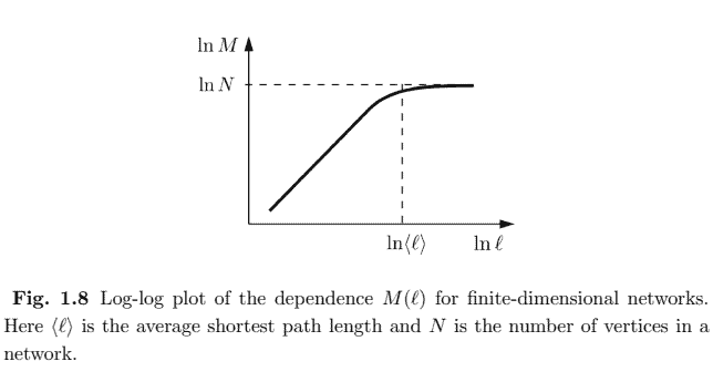
The space dimension $D$, introduced in this way, coincides with the Hausdorff dimension in many interesting for us networks, and so we loosely use the latter term as physicists often do (Durhuus, 2009). For a finite network, we can introduce the distribution $\mathcal{P}(\ell)$ of the lengths of the shortest paths connecting the pairs of vertices, the first moment of this distribution, that is, the average shortest path distance $\langle\ell\rangle$, and the diameter of the network, $d=\max (\ell)$, that is, the maximum separation of two vertices in the network. For a large, though finite, lattice of $N$ vertices, the power-law dependence $M(\ell)$, Eq. (1.7) approaches the upper limit $N$ when $\ell \sim d \sim\langle\ell\rangle$ (Figure 1.8), so
$$
N \sim d^{D} \sim\langle\ell\rangle^{D} .
$$
Therefore, the mean separation of vertices in finite-dimensional lattices is large in the sense that it increases with $N$ in a power-law way,
$$
\langle\ell\rangle(N) \sim N^{1 / D}
$$
数据科学代写|复杂网络代写Complex Network代考|First structural characteristics of networks
One can introduce local and global structural characteristics of a graph. Let us start from the local ones, which are for individual vertices and use only local information. We assume that networks are undirected, that is, their edges are not oriented. The first natural characteristic is the degree of a given vertex $i$ in a graph. This is the number $q_{i}$ of the edge ends attached to this vertex. For example, if a vertex has only a self-loop (1-cycle), then its degree equals 2, although this vertex is incident to a single edge. The next quantity, local clustering, characterizes the set of connections between the nearest neighbours of a vertex $i$. This is the ratio of the number $t_{i}$ of edges between the nearest neighbours of vertex $i$ and the maximum possible number of such connections, namely,
$$
C_{i}=\frac{t_{i}}{q_{i}\left(q_{i}-1\right) / 2},
$$
so $C_{i} \leq 1$. Here, $t_{i}$ is also the number of triangles attached to vertex $i$, and the denominator $q_{i}\left(q_{i}-1\right) / 2$ is the maximum possible number of such triangles (cycles of length 3 ). 10
Introducing the shortest path distance $\ell_{i j}$ between two vertices, $i$ and $j$, which depends on how connections are organized in a part of this graph between $i$ and $j$, enables us to define the diameter $d=\max {i, j} \ell{i j}$ characterizing the entire graph. The diameter is an example of a global structural characteristic. Note that this characteristic is useful only if the biggest connected component in a graph is large compared to other its connected components.
The statistics of degrees in a random network is provided by the degree distribution,
$$
P(q)=\left\langle\frac{N(q)}{N}\right\rangle=\left\langle\frac{1}{N} \sum_{i} \delta\left(q_{i}, q\right)\right\rangle
$$
where $N$ is the number of vertices in a graph-a member of the statistical ensemble (this number can be different in different members of the ensembles), $N(q)$ is the number of vertices of degree $q$ in this graph, and $\langle\ldots\rangle$ denotes averaging over the ensemble, explained in Section 1.1.11 $\delta\left(q_{i}, q\right) \equiv \delta_{q_{i}, q}$ is the Kronecker symbol. The moments of this distribution are
$$
\left\langle q^{n}\right\rangle=\left\langle\frac{1}{N} \sum_{i} q_{i}^{n}\right\rangle=\sum_{q} P(q) q^{n}
$$
复杂网络代写
数据科学代写|复杂网络代写COMPLEX NETWORK代考|SMALL AND LARGE WORLDS
大型网絡的关键特征inparticular, alargelattice 是它的空间维数,即允许指定网络中任何顶点的最小坐标数。我们从一个简单的考虑开始,将细节留到后面的章 节。考虑一个无限规则,例如,具有单位长度边的超立方、有限维晶格。选择一些它的顶点和远处的所有顶点或更小。距离测量为计算路径中边数的两个顶点之 间的最短路径的长度。那么顶点数 $M(\ell)$ 在这个球增加作为力量 $\ell$,
$$
M(\ell) \sim \ell^{D}
$$
对于大 $\ell$ ,和
$$
D=\frac{d \ln M(\ell)}{d \ln \ell} .
$$ 话说,系统的行为可能对运动方程的形式极为敏感,运动方程的微小变化会导致系统行为的巨大变化。马克纽曼2011提出了另一个定义:“复杂系统是由许多相互 作用的部分组成的系统,通常称为代理,它表现出集体行为,而不是从各个部分的行为中简单地逻循。,
空间维度 D,以这种方式引入,与许多我们感兴趣的网络中的 Hausdorff 维相吻合,因此我们像物理学家经常做的那样松散地使用后一个术语 Durhuus, 2009. 对 于有限网络,我们可以引入分布 $\mathcal{P}(\ell)$ 连接顶点对的最短路径的长度,这个分布的一阶矩,即平均最短路径距离 $(\ell)$ ,以及网络的直径, $d=\max (\ell)$ ,即网络中两个 顶点的最大间隔。对于一个大的但有限的晶格 $N$ 顶点,龺律依赖 $M(\ell)$, 方程。 $1.7$ 接近上限 $N$ 什么时候 $\ell \sim d \sim\langle\ell\rangle F i g u r e 1.8$ ,所以
$$
N \sim d^{D} \sim\langle\ell\rangle^{D} .
$$
因此,在有限维格子中顶点的平均间隔是很大的,因为它随着它的增加而增加 $N$ 以冥律方式,
$$
\langle\ell\rangle(N) \sim N^{1 / D}
$$
数据科学代写|复杂网络代写COMPLEX NETWORK代考|FIRST STRUCTURAL CHARACTERISTICS OF NETWORKS
可以引入图的局部和全局结构特征。让我们从局部顶点开始,它们用于单个顶点并且仅使用同部信息。我们假设网絡是无向的,也就是说,它们的边缘是无向的。 第一个自然特征是给定顶点的度数 $i$ 在图表中。这是号码 $q_{i}$ 连接到该顶点的边的端点。例如,如果一个顶点只有一个自环 $1-c y c l e$ ,那么它的度数等于 2 ,尽管这 个顶点是与单个边相关的。下一个量,局部聚类,表征顶点最近邻居之间的连接集 $i$. 这是数字的比例 $t_{i}$ 顶点最近邻居之间的边数 $i$ 以及此类连接的最大可能数量,即
$$
C_{i}=\frac{t_{i}}{q_{i}\left(q_{i}-1\right) / 2}
$$
所以 $C_{i} \leq 1$. 这里, $t_{i}$ 也是连接到顶点的三角形的数量 $i$, 和分母 $q_{i}\left(q_{i}-1\right) / 2$ 是此类三角形的最大可能数量 $c y c l e s o f l e n g t h 3.10$
引入最短路径距离 $\ell_{i j}$ 两个顶点之间, $i$ 和 $j$ ,这取决于连接在该图中的一部分之间的组织方式 $i$ 和 $j$ ,使我们能够定义直径 $d=\max i, j \ell i j$ 表征整个图形。直径是全局 结构特征的一个例子。请注意,仅当图中最大的连通分量与其他连通分量相比较大时,此特性才有用。 随机网絡中度数的统计由度数分布提供,
$$
P(q)=\left\langle\frac{N(q)}{N}\right\rangle=\left\langle\frac{1}{N} \sum_{i} \delta\left(q_{i}, q\right)\right\rangle
$$
在哪里 $N$ 是图中的顶点数 – 统计集成的成员thisnumbercanbedifferentindifferentmembersoftheensembles, $N(q)$ 是度数的顶点数 $q$ 在该图中,并且 〈… 表
$$
\left\langle q^{n}\right\rangle=\left\langle\frac{1}{N} \sum_{i} q_{i}^{n}\right\rangle=\sum_{q} P(q) q^{n}
$$

数据科学代写|复杂网络代写Complex Network代考 请认准UprivateTA™. UprivateTA™为您的留学生涯保驾护航。
微观经济学代写
微观经济学是主流经济学的一个分支,研究个人和企业在做出有关稀缺资源分配的决策时的行为以及这些个人和企业之间的相互作用。my-assignmentexpert™ 为您的留学生涯保驾护航 在数学Mathematics作业代写方面已经树立了自己的口碑, 保证靠谱, 高质且原创的数学Mathematics代写服务。我们的专家在图论代写Graph Theory代写方面经验极为丰富,各种图论代写Graph Theory相关的作业也就用不着 说。
线性代数代写
线性代数是数学的一个分支,涉及线性方程,如:线性图,如:以及它们在向量空间和通过矩阵的表示。线性代数是几乎所有数学领域的核心。
博弈论代写
现代博弈论始于约翰-冯-诺伊曼(John von Neumann)提出的两人零和博弈中的混合策略均衡的观点及其证明。冯-诺依曼的原始证明使用了关于连续映射到紧凑凸集的布劳威尔定点定理,这成为博弈论和数学经济学的标准方法。在他的论文之后,1944年,他与奥斯卡-莫根斯特恩(Oskar Morgenstern)共同撰写了《游戏和经济行为理论》一书,该书考虑了几个参与者的合作游戏。这本书的第二版提供了预期效用的公理理论,使数理统计学家和经济学家能够处理不确定性下的决策。
微积分代写
微积分,最初被称为无穷小微积分或 “无穷小的微积分”,是对连续变化的数学研究,就像几何学是对形状的研究,而代数是对算术运算的概括研究一样。
它有两个主要分支,微分和积分;微分涉及瞬时变化率和曲线的斜率,而积分涉及数量的累积,以及曲线下或曲线之间的面积。这两个分支通过微积分的基本定理相互联系,它们利用了无限序列和无限级数收敛到一个明确定义的极限的基本概念 。
计量经济学代写
什么是计量经济学?
计量经济学是统计学和数学模型的定量应用,使用数据来发展理论或测试经济学中的现有假设,并根据历史数据预测未来趋势。它对现实世界的数据进行统计试验,然后将结果与被测试的理论进行比较和对比。
根据你是对测试现有理论感兴趣,还是对利用现有数据在这些观察的基础上提出新的假设感兴趣,计量经济学可以细分为两大类:理论和应用。那些经常从事这种实践的人通常被称为计量经济学家。
Matlab代写
MATLAB 是一种用于技术计算的高性能语言。它将计算、可视化和编程集成在一个易于使用的环境中,其中问题和解决方案以熟悉的数学符号表示。典型用途包括:数学和计算算法开发建模、仿真和原型制作数据分析、探索和可视化科学和工程图形应用程序开发,包括图形用户界面构建MATLAB 是一个交互式系统,其基本数据元素是一个不需要维度的数组。这使您可以解决许多技术计算问题,尤其是那些具有矩阵和向量公式的问题,而只需用 C 或 Fortran 等标量非交互式语言编写程序所需的时间的一小部分。MATLAB 名称代表矩阵实验室。MATLAB 最初的编写目的是提供对由 LINPACK 和 EISPACK 项目开发的矩阵软件的轻松访问,这两个项目共同代表了矩阵计算软件的最新技术。MATLAB 经过多年的发展,得到了许多用户的投入。在大学环境中,它是数学、工程和科学入门和高级课程的标准教学工具。在工业领域,MATLAB 是高效研究、开发和分析的首选工具。MATLAB 具有一系列称为工具箱的特定于应用程序的解决方案。对于大多数 MATLAB 用户来说非常重要,工具箱允许您学习和应用专业技术。工具箱是 MATLAB 函数(M 文件)的综合集合,可扩展 MATLAB 环境以解决特定类别的问题。可用工具箱的领域包括信号处理、控制系统、神经网络、模糊逻辑、小波、仿真等。