如果你也在 怎样代写统计入门Introduction to Statistics KMA153这个学科遇到相关的难题,请随时右上角联系我们的24/7代写客服。广义线性模型Generalized linear model是一门涉及数据的收集、组织、分析、解释和表述的学科。在将统计学应用于科学、工业或社会问题时,通常会从一个统计人口或一个待研究的统计模型开始。人口可以是不同的人群或物体,如 “生活在一个国家的所有人 “或 “组成一个晶体的每个原子”。统计学涉及数据的方方面面,包括设计调查和实验方面的数据收集计划。
统计入门Introduction to Statistics在数据分析中主要使用两种统计方法:描述性统计和推断性统计,前者使用平均数或标准差等指标对样本数据进行总结,后者从受随机变化影响的数据中得出结论(例如。描述性统计最常关注的是分布(样本或人群)的两组属性:中心倾向(或位置)试图描述分布的中心或典型值,而分散性(或变异性)则描述分布中的成员偏离其中心和彼此的程度。对数学统计的推断是在概率论的框架下进行的,概率论涉及到对随机现象的分析。
统计入门Introduction to Statistics代写,免费提交作业要求, 满意后付款,成绩80\%以下全额退款,安全省心无顾虑。专业硕 博写手团队,所有订单可靠准时,保证 100% 原创。最高质量的统计入门Introduction to Statistics作业代写,服务覆盖北美、欧洲、澳洲等 国家。 在代写价格方面,考虑到同学们的经济条件,在保障代写质量的前提下,我们为客户提供最合理的价格。 由于作业种类很多,同时其中的大部分作业在字数上都没有具体要求,因此统计入门Introduction to Statistics作业代写的价格不固定。通常在专家查看完作业要求之后会给出报价。作业难度和截止日期对价格也有很大的影响。
同学们在留学期间,都对各式各样的作业考试很是头疼,如果你无从下手,不如考虑my-assignmentexpert™!
my-assignmentexpert™提供最专业的一站式服务:Essay代写,Dissertation代写,Assignment代写,Paper代写,Proposal代写,Proposal代写,Literature Review代写,Online Course,Exam代考等等。my-assignmentexpert™专注为留学生提供Essay代写服务,拥有各个专业的博硕教师团队帮您代写,免费修改及辅导,保证成果完成的效率和质量。同时有多家检测平台帐号,包括Turnitin高级账户,检测论文不会留痕,写好后检测修改,放心可靠,经得起任何考验!
想知道您作业确定的价格吗? 免费下单以相关学科的专家能了解具体的要求之后在1-3个小时就提出价格。专家的 报价比上列的价格能便宜好几倍。
统计代写|统计入门代写Introduction to Statistics代考|What Is the Most Direct Way to Interpret the Value of a Correlation Coefficient?
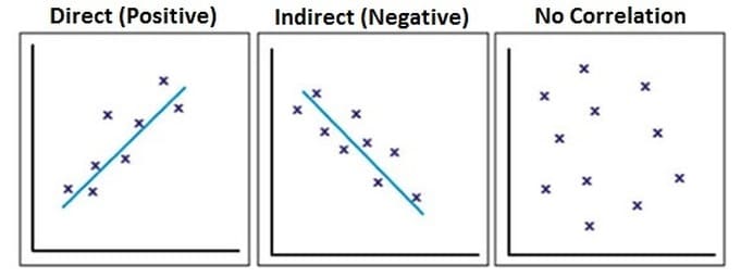
The correlation coefficient is a numerical value that indicates the degree of relationship between two variables. The value of any correlation coefficient ranges from $-1.00$ (a perfectly indirect or negative correlation) to $+1.00$ (a perfectly direct or positive correlation). But how does one interpret this value? What does it mean?
The most direct way to interpret a correlation coefficient is to use the following table. This will give you a quick assessment of the strength of the correlation.
While using the above table is not the most precise way of interpreting the strength of a correlation coefficient, it certainly provides a sense of the strength of the relationship between variables. For a more precise method, we’ll turn to question $# 47$, which deals with the coefficient of determination.
统计代写|统计入门代写Introduction to Statistics代考|What Is the Coefficient of Determination, and How Is It Computed?
Ithough a simple examination of the value of a correlation coefficient can provide a general assessment of the strength of the relationship between two variables, there is a far more precise way to do this.
The coefficient of determination, represented as $r_{x y}{ }^2$ or the square of the correlation coefficient, yields the amount of variance in one variable that is accounted for by changes in another variable. The concept of the coefficient of determination is based on the fact that variables that are correlated with one another share something in common. The stronger the relationship $\left(r_{x y}\right)$, the more they share and the higher the coefficient of determination.
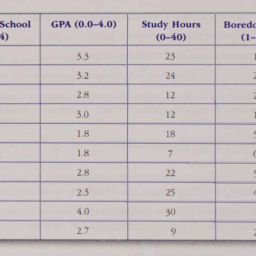
For example, let’s take the correlation between height and weight for a class of sixth graders, which is found to be 85 . Thus, the simple Pearson product-moment correlation or $r_{x y}=.85$. The coefficient of determination is $.7225$, which means that $72.25 \%$ of the variance in height (how much sixth graders differ from each other in height) can be accounted for by the variance in weight (how much sixth graders differ from each in weight).
There are several important things to remember about the use of this coefficient.
The first is that the stronger the simple correlation, the more variance is accounted for. For example, if the correlation between one variable and the other is $.4$, then only 16 or $16 \%$ of the variance in one is accounted for by the relationship between variables. If the correlation between one variable and another is $.6$, then $.36$ or $36 \%$ of the variance is accounted for.
The second (related to the first) is that the more that one variable has in common with a second variable (and the stronger the correlation), the larger the coefficient of determination will be.
If there is no relationship between variables (when $r_{x y}=0$ ), then nothing is shared between the two variables, and no variance or change in one can be accounted for by a change in the other.
Indirect or negative correlations, which have a negative sign (such as $-.13$ or $-.87$ ) are neither “better” nor “worse” than direct or positive correlation coefficients-just very different.
A correlation always reflects a situation in which there are at least two data points (or variables) per case.
A correlation indicates nothing about the causal relationship between variables; it reflects only the strength of their association.
Scatter charts are the best choice to display the visual relationship between points whose correlation is being explored.
统计入门代写
统计代写|统计入门代写INTRODUCTION TO STATISTICS代 考|WHAT IS THE MOST DIRECT WAY TO INTERPRET THE VALUE OF A CORRELATION COEFFICIENT?
相关系数是表示两个变量之间相关程度的数值。任何相关系数的值范围为-1.00 aper fectlyindirectornegativecorrelation至 $+1.00$ aper fectlydirectorpositivecorrelation. 但是如何解释这个值呢? 这是什么意思?
解释相关系数最直接的方法是使用下表。这将使您快速评估相关性的强度。
虽然使用上表并不是解释相关系数强度的最精确方式,但它确实提供了对变量之间关系强度的感觉。对于更精确的方法,我们将转向问题#47,它处理决定系数。
统计代写|统计入门代写INTRODUCTION TO STATISTICS代 考|WHAT IS THE COEFFICIENT OF DETERMINATION, AND HOW IS IT COMPUTED?
屈管对相关系数值的简单检柦可以提供对两个变量之间关系强度的一般评估,但有一种更精确的方法可以做到这一点。
决定系数,表示为 $r_{x y}{ }^2$ 或相关系数的平方,产生一个变量的方差量,该变量由另一个变量的变化来解释。决定系数的概念基于这样一个事实,即彼此相关的变量具 有共同点。关系越强 $\left(r_{x y}\right)$ ,他们分享的越多,决定系数就越高。
例如,让我们以一个六年级学生的身高和体重之间的相关性为例,发现它是 85 。因此,简单的 Pearson 积矩相关或 $r_{x y}=.85$. 决定系数为. 7225 ,意思就是
$72.25 \%$ 高度的变化howmuchsixthyradersdifferfromeachotherinheight可以通过重量的变化来解释howmuchsixthgradersdiffer fromeachinweight.
关于这个系数的使用,有几件重要的事情需要记住。
首先是简单相关性越强,解释的方差就越多。例如,如果一个变量与另一个变量之间的相关性为. 4 , 那么只有 16 或 $16 \%$ 变量之间的关系可以解释变量之间的差异。 如果一个变量和另一个变量之间的相关性是.6,然后.36或者 $36 \%$ 的差异被考虑在内。
第二relatedtothe first二个变量与第二个变量的共同点越多 andthestrongerthecorrelation,决定系数越大。
如果变量之间没有关系 $w h e n \$ r_{x y}=0 \$$ ,则两个变量之间没有任何共享,并且一个变量的变化或变化不能由另一个变量的变化来解释。
具有负昊的间接或负相关suchas\$-.13\$or $\$-.87 \$$ 既不比直接或正相关系数“好”也不“差”一只是非常不同。
相关性总是反映至少有两个数据点的情况orvariables每个案例。
相关性表明变量之间没有因果关系;它只反映了他们协会的力量。
散点图是显示正在探索相关性的点之间的视觉关系的最佳选择。

统计代写|统计入门代写INTRODUCTION TO STATISTICS代考 请认准UprivateTA™. UprivateTA™为您的留学生涯保驾护航。
微观经济学代写
微观经济学是主流经济学的一个分支,研究个人和企业在做出有关稀缺资源分配的决策时的行为以及这些个人和企业之间的相互作用。my-assignmentexpert™ 为您的留学生涯保驾护航 在数学Mathematics作业代写方面已经树立了自己的口碑, 保证靠谱, 高质且原创的数学Mathematics代写服务。我们的专家在图论代写Graph Theory代写方面经验极为丰富,各种图论代写Graph Theory相关的作业也就用不着 说。
线性代数代写
线性代数是数学的一个分支,涉及线性方程,如:线性图,如:以及它们在向量空间和通过矩阵的表示。线性代数是几乎所有数学领域的核心。
博弈论代写
现代博弈论始于约翰-冯-诺伊曼(John von Neumann)提出的两人零和博弈中的混合策略均衡的观点及其证明。冯-诺依曼的原始证明使用了关于连续映射到紧凑凸集的布劳威尔定点定理,这成为博弈论和数学经济学的标准方法。在他的论文之后,1944年,他与奥斯卡-莫根斯特恩(Oskar Morgenstern)共同撰写了《游戏和经济行为理论》一书,该书考虑了几个参与者的合作游戏。这本书的第二版提供了预期效用的公理理论,使数理统计学家和经济学家能够处理不确定性下的决策。
微积分代写
微积分,最初被称为无穷小微积分或 “无穷小的微积分”,是对连续变化的数学研究,就像几何学是对形状的研究,而代数是对算术运算的概括研究一样。
它有两个主要分支,微分和积分;微分涉及瞬时变化率和曲线的斜率,而积分涉及数量的累积,以及曲线下或曲线之间的面积。这两个分支通过微积分的基本定理相互联系,它们利用了无限序列和无限级数收敛到一个明确定义的极限的基本概念 。
计量经济学代写
什么是计量经济学?
计量经济学是统计学和数学模型的定量应用,使用数据来发展理论或测试经济学中的现有假设,并根据历史数据预测未来趋势。它对现实世界的数据进行统计试验,然后将结果与被测试的理论进行比较和对比。
根据你是对测试现有理论感兴趣,还是对利用现有数据在这些观察的基础上提出新的假设感兴趣,计量经济学可以细分为两大类:理论和应用。那些经常从事这种实践的人通常被称为计量经济学家。
Matlab代写
MATLAB 是一种用于技术计算的高性能语言。它将计算、可视化和编程集成在一个易于使用的环境中,其中问题和解决方案以熟悉的数学符号表示。典型用途包括:数学和计算算法开发建模、仿真和原型制作数据分析、探索和可视化科学和工程图形应用程序开发,包括图形用户界面构建MATLAB 是一个交互式系统,其基本数据元素是一个不需要维度的数组。这使您可以解决许多技术计算问题,尤其是那些具有矩阵和向量公式的问题,而只需用 C 或 Fortran 等标量非交互式语言编写程序所需的时间的一小部分。MATLAB 名称代表矩阵实验室。MATLAB 最初的编写目的是提供对由 LINPACK 和 EISPACK 项目开发的矩阵软件的轻松访问,这两个项目共同代表了矩阵计算软件的最新技术。MATLAB 经过多年的发展,得到了许多用户的投入。在大学环境中,它是数学、工程和科学入门和高级课程的标准教学工具。在工业领域,MATLAB 是高效研究、开发和分析的首选工具。MATLAB 具有一系列称为工具箱的特定于应用程序的解决方案。对于大多数 MATLAB 用户来说非常重要,工具箱允许您学习和应用专业技术。工具箱是 MATLAB 函数(M 文件)的综合集合,可扩展 MATLAB 环境以解决特定类别的问题。可用工具箱的领域包括信号处理、控制系统、神经网络、模糊逻辑、小波、仿真等。