MY-ASSIGNMENTEXPERT™可以为您提供 sydney BSTA5009 Survival Models 生存模型的代写代考和辅导服务!
这是悉尼大学 生存模型课程的代写成功案例。

BSTA5009课程简介
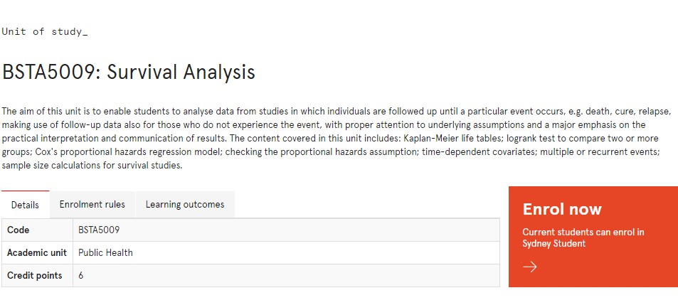
The aim of this unit is to enable students to analyse data from studies in which individuals are followed up until a particular event occurs, e.g. death, cure, relapse, making use of follow-up data also for those who do not experience the event, with proper attention to underlying assumptions and a major emphasis on the practical interpretation and communication of results. The content covered in this unit includes: Kaplan-Meier life tables; logrank test to compare two or more groups; Cox’s proportional hazards regression model; checking the proportional hazards assumption; time-dependent covariates; multiple or recurrent events; sample size calculations for survival studies.
Prerequisites
At the completion of this unit, you should be able to:
- LO1. Understand the nature of survival data
- LO2. Summarise and display survival data using nonparametric methods
- LO3. Analyse survival data using the Cox proportional hazards model, including time-dependent covariates
- LO4. Analyse survival data using parametric models
- LO5. Analyse data using multi-event models
- LO6. Determine sample size for simple survival analysis
- LO7. Produce appropriate displays for publication
BSTA5009 Survival Models HELP(EXAM HELP, ONLINE TUTOR)
In a certain life table, $\ell_x=1000$ and $\ell_{x+1}=900$. Evaluate $m_x$ under each of the UDD, constant force, and Balducci assumptions.
SOLUTION From the given values we find $d_x=100, \ln p_x=-.10536$, and $\mu=-\ln p_x=.10536$. Under UDD, $L_x=\ell_x-\frac{1}{2} d_x=950$, so we obtain $m_x=\frac{d_x}{L_x}=.10526$; under constant force, we directly have $m_x=\mu=.10536$; under Balducci, $L_x=\frac{-\ell_{x+1} \cdot \ln p_x}{q_x}=948.24$, so $m_x=\frac{100}{948.24}=.10545$.
Express the conditional probabilities (a) ${ }{2 \mid 4} q{[20]+1}$ and (b) ${ }{2 \mid 4} q{[22]+3}$ in terms of $\ell$ ‘s, assuming a 4-year select period.
SOLUTION
(a) This is the probability of death between ages 23 and 27 for a person age 21 , selected at age 20 . The number of such deaths, from Table 3.5, is $\ell_{[20]+3}-\ell_{27}$, so the desired probability is $\frac{\ell_{[200+3}-\ell_{27}}{\ell_{[20]+1}}$.
(b) Here we seek the probability of death between ages 27 and 31 for a person age 25 , selected at age 22 . For this person, age 27 is already beyond the select period, so the probability is $\frac{\ell_{27}-\ell_{31}}{\ell_{[22]+3}}$.
In this section we have developed the select and ultimate life table from values of $S(t ; x)$. Alternatively, a set of $q_{[x]+t}, t=0,1,2,3$, for all ages at selection, and $q_{x+t}, t \geq 4$, might be available. Since $p_{[x]+t}=1-q_{[x]+t}$ and $p_{x+1}=1-q_{x+t}$, then values of $S(t ; x)$ can easily be found. Thus the development of a select life table from a set of $q$ ‘s is totally parallel to its development from $S(t ; x)$. For a description of this select table development from $q$ ‘s, specifically oriented to the idea of selection for issuance of insurance, see Section 1.8 of Jordan [41].
A cohort of eight individuals is observed from time $t=0$ until all have failed. Only the day of failure is recorded. (By assuming that the initial event defining $t=0$ occurs in the middle of the day, and failure also occurs in the middle of the day, then all durations at failure are integral.) The observed durations at failure were $3,4,5,5,7,10,10,12$. The observed proportion of the sample surviving, $S^o(t)$, is used to estimate the operative (but unknown) $S(t)$. (a) What are our estimates of $S(2), S(5)$, and $S(12)$ ? (b) Graph $S^{\circ}(t)$.
(a) $S^o(2)=1.00$, the proportion still surviving. Since we have defined $S^o(t)$ to be right continuous, by (4.1), the observed proportion surviving at $t=5$ is $S^o(5)=.50$. Similarly, since $t_8=12$ is the time of the last death, then $S^o(12)=0$.
In general, we might use the procedure of this section for cohorts small enough to avoid a prohibitive amount of computation. For larger samples, we can use the approach described in Section 4.4.
Suppose it is known that the survival distribution to which our sample in Example 4.2 is actually subject is uniform on $(0,15]$. (a) What is the variance of the random variable $S^o(6)$ ? (b) If the uniform distribution assumption is not made, how would we estimate $\operatorname{Var}\left[S^{\circ}(6)\right]$ ?
SOLUTION
(a) If $T$ is uniform on $(0,15]$, then $S(6)=.60$ and $\operatorname{Var}\left[S^{\circ}(6)\right]=\frac{(.6)(.4)}{8}=.03$.
(b) Note that $S^{\circ}(6)=.50$, so $(4.5)$ gives est. $\operatorname{Var}\left[S^{\circ}(6)\right]=\frac{(.5)(.5)}{8}=.03125$. [Note: The data of this sample could be used to test the hypothesis that the applicable distribution is uniform on $(0,15]$. We will do this in Chapter 8.]
MY-ASSIGNMENTEXPERT™可以为您提供 sydney BSTA5009 Survival Models 生存模型的代写代考和辅导服务!


