UpriviateTA代写,做自己擅长的领域!UpriviateTA的专家精通各种经典论文、方程模型、通读各种完整书单,比如代写和线性代数密切相关的Matrix theory, 各种矩阵形式的不等式,比如Wely inequality, Min-Max principle,polynomial method, rank trick那是完全不在话下,对于各种singularity value decomposition, LLS, Jordan standard form ,QR decomposition, 基于advance的LLS的optimazation问题,乃至于linear programming method(8维和24维Sphere packing的解决方案的关键)的计算也是熟能生巧正如一些大神所说的,代写线性代数留学生线性代数作业assignment论文paper的很多方法都是围绕几个线性代数中心问题的解决不断产生的。比如GIT,从klein时代开始研究的几何不变量问题,以及牛顿时代开始研究的最优化问题等等(摆线),此外,强烈推荐我们UpriviateTA代写的线性代数这门课,从2017年起,我们已经陆续代写过近千份类似的作业assignment。 以下就是一份典型案例的答案
问题 1. Let \(A\) be a real matrix. If there exists an orthogonal matrix \(Q\) such that \(A=Q\left[\begin{array}{l}R \\ 0\end{array}\right],\) show that
$$
A^{T} A=R^{T} R
$$
证明 . This simply involves multiplying the block matrices out:
$$
A^{T} A=\left[\begin{array}{ll}
R^{T} & 0
\end{array}\right] Q^{T} Q\left[\begin{array}{l}
R \\
\end{array}\right]=\left[\begin{array}{ll}
R^{T} & 0
\end{array}\right]\left[\begin{array}{l}
R \\
\end{array}\right]=R^{T} R
$$
问题 2. Let \(A\) be symmetric positive definite. Given an initial guess \(x_{0},\) the method of steepest descent for solving \(A x=b\) is defined as
$$
x_{k+1}=x_{k}+\alpha_{k} r_{k}
$$
where \(r_{k}=b-A x_{k}\) and \(\alpha_{k}\) is chosen to minimize \(f\left(x_{k+1}\right),\) where
$$
f(x):=\frac{1}{2} x^{T} A x-x^{T} b
$$
(a) Show that
$$
\alpha_{k}=\frac{r_{k}^{T} r_{k}}{r_{k}^{T} A r_{k}}
$$
(b) Show that
$$
r_{i+1}^{T} r_{i}=0
$$
(c) If \(e_{i}:=x-x_{i} \neq 0,\) show that
$$
e_{i+1}^{T} A e_{i+1}<e_{i}^{T} A e_{i}
$$
Hint: This is equivalent to showing \(r_{i+1}^{T} A^{-1} r_{i+1}<r_{i}^{T} A^{-1} r_{i}\) (why?).
证明 . (a) To find out what \(\alpha_{k}\) is, apply the recurrence relation to the definition of \(f\left(x_{k+1}\right)\) :
\(\begin{aligned} f\left(x_{k+1}\right) &=\frac{1}{2}\left(x_{k}+\alpha_{k} r_{k}\right)^{T} A\left(x_{k}+\alpha_{k} r_{k}\right)-\left(x_{k}+\alpha_{k} r_{k}\right)^{T} b \\ &=\frac{1}{2}\left(x_{k}^{T} A x_{k}+\alpha_{k} r_{k}^{T} A x_{k}+\alpha_{k} x_{k}^{T} A r_{k}+\alpha_{k}^{2} r_{k}^{T} A r_{k}\right)-x_{k}^{T} b-\alpha_{k} r_{k}^{T} b \\ &=\frac{1}{2}\left(x_{k}^{T} A x_{k}+\alpha_{k} r_{k}^{T} A x_{k}+\alpha_{k} r_{k}^{T} A^{T} x_{k}+\alpha_{k}^{2} r_{k}^{T} A r_{k}\right)-x_{k}^{T} b-\alpha_{k} r_{k}^{T} b \\ &=\frac{1}{2}\left(x_{k}^{T} A x_{k}+\alpha_{k} r_{k}^{T} A x_{k}+\alpha_{k} r_{k}^{T} A x_{k}+\alpha_{k}^{2} r_{k}^{T} A r_{k}\right)-x_{k}^{T} b-\alpha_{k} r_{k}^{T} b \\ &=\frac{1}{2}\left(x_{k}^{T} A x_{k}+2 \alpha_{k} r_{k}^{T} A x_{k}+\alpha_{k}^{2} r_{k}^{T} A r_{k}\right)-x_{k}^{T} b-\alpha_{k} r_{k}^{T} b \end{aligned}\)
Now differentiate with respect to \(\alpha_{k}\) and set to zero:
$$
\begin{aligned}
\frac{d}{d \alpha_{k}} f\left(x_{k+1}\left(\alpha_{k}\right)\right) &=r_{k}^{T} A x_{k}+\alpha r_{k}^{T} A r_{k}-r_{k}^{T} b=0 \\
\alpha_{k} r_{k}^{T} A r_{k} &=r_{k}^{T} b-r_{k}^{T} A x_{k}=r_{k}^{T} r_{k}
\end{aligned}
$$
Isolating \(\alpha_{k}\) yields the desired result. Note that \(\alpha>0,\) since \(A\) is positive definite.
(b) It helps to first establish a recurrence relation involving the residuals only: note that
$$
r k+1=b-A x_{k+1}=b-A\left(x_{k}+\alpha_{k} r_{k}\right)=r_{k}-\alpha_{k} A r_{k}
$$
Then
$$
\begin{aligned}
r_{k+1}^{T} r_{k} &=\left(r_{k}-\alpha_{k} A r_{k}\right)^{T} r_{k} \\
&=r_{k}^{T} r_{k}-\left(\frac{r_{k}^{T} r_{k}}{r_{k}^{T} A r_{k}}\right) r_{k}^{T} A^{T} r_{k} \\
&=0
\end{aligned}
$$
since \(A=A^{T}\).
(c) First, note that
$$
r_{k}=b-A x_{k}=A x-A x_{k}=A\left(x-x_{k}\right)=A e_{k}
$$
so that \(r_{k}^{T} A^{-1} r_{k}=e_{k}^{T} A^{T} A^{-1} A e_{k}=e_{k}^{T} A e_{k},\) and similarly for \(r_{k+1}\). Thus, the two inequalities are completely equivalent. Now we attack the inequality involving \(r\) :
$$
\begin{aligned}
r_{k+1}^{T} A^{-1} r_{k+1} &=r_{k+1}^{T} A^{-1}\left(r_{k}-\alpha_{k} A r_{k}\right) \\
&=r_{k+1}^{T} A^{-1} r_{k}-\underbrace{\alpha_{k} r_{k+1}^{T} r_{k}}_{0 \text { by (b) }} \\
&=\left(r_{k}-\alpha_{k} A r_{k}\right)^{T} A^{-1} r_{k} \\
&=r_{k} A^{-1} r_{k}-\underbrace{\alpha_{k} r_{k}^{T} r_{k}}_{>0} \\
&<r_{k} A^{-1} r_{k} .
\end{aligned}
$$
问题 3. Let \(B\) be an \(n \times n\) matrix, and assume that \(B\) is both orthogonal and triangular.
(a) Prove that \(B\) must be diagonal.
(b) What are the diagonal entries of \(B ?\)
(c) Let \(A\) be \(n \times n\) and non-singular. Use parts (a) and (b) to prove that the QR factorization of \(A\) is unique up to the signs of the diagonal entries of \(R\). In particular, show that there exist unique matrices \(Q\) and \(R\) such that \(Q\) is orthogonal, \(R\) is upper triangular with positive entries on its main diagonal, and \(A=Q R\).
证明 . Solution. (a) We need two facts:
i. \(P, Q\) orthogonal \(\Longrightarrow P Q\) orthogonal
ii. \(P\) upper triangular \(\Longrightarrow P^{-1}\) upper triangular
(i) is easy: \((P Q)^{T}(P Q)=Q^{T} P^{T} P Q=Q^{T} I Q=Q^{T} Q=I\).
(ii) can be argued by considering the \(k\) th column \(p_{k}\) of \(P^{-1}\). Then \(P^{-1} e_{k}=p_{k},\) so \(P p_{k}=e_{k}\). Since \(P\) is upper triangular, we can use backward substitution to solve for \(p_{k} .\) Recall the formula for backward substitution for a general upper triangular system \(T x=b\) :
$$
x_{k}=\frac{1}{t_{k k}}\left(b_{k}-\sum_{j=k+1}^{n} t_{k j} b_{j}\right)
$$
In our case, we see that since \(\left(e_{k}\right)_{j}=0\) for \(j>k,\) this implies \(\left(p_{k}\right)_{j}=0\) for \(j>k .\) In other words, the \(k\) th column of \(P^{-1}\) must be all zero below the \(k\) th row. This is to say \(P^{-1}\) is upper triangular. Now we show that \(B\) both orthogonal and triangular implies \(B\) diagonal. Without loss of generality (i.e. replacing \(B\) by \(B^{T}\) if necessary), we can assume \(B\) is upper triangular. Then \(B^{-1}\) is also upper triangular by (ii). But \(B^{-1}=B^{T}\) by orthogonality, and we know \(B^{T}\) is lower triangular. So \(B^{T}\) (and hence \(B\) ) is both upper and lower triangular, implying that \(B\) is in fact diagonal.
(b) We know \(B\) is diagonal, so that \(B=B^{T} .\) Let \(B=\operatorname{diag}\left(b_{11}, \ldots, b_{n n}\right) .\) Then \(I=B B^{T}=\) \(\operatorname{diag}\left(b_{11}^{2}, \ldots, b_{n n}^{2}\right),\) so \(b_{i i}^{2}=1\) for all \(i .\) Thus, the diagonal entries of \(B\) are \(\pm 1 .\)
(c) There is an existence part and a uniqueness part to this problem. In class we showed existence of a decomposition \(A=Q R\) where \(Q\) is orthogonal, and \(R\) is upper triangular, but not necessarily with positive entries on the diagonal, so we have to fix it up. We know that \(r_{i i} \neq 0\) (otherwise \(R\) would be singular, contradicting the non-singularity of \(A\) ), so we can define
$$
D=\operatorname{diag}\left(\operatorname{sgn}\left(r_{11}\right), \ldots, \operatorname{sgn}\left(r_{n n}\right)\right)
$$
where
$$
\operatorname{sgn}(x)=\left\{\begin{array}{ll}
1, & x>0 \\
0, & x=0 \\
-1, & x<0
\end{array}\right.
$$
Note that \(D\) is orthogonal, and \(\tilde{R}=D R\) has positive diagonal. So if we define \(\tilde{Q}=Q D\) (orthogonal), then \(A=\tilde{Q} \tilde{R}\) gives the required decomposition, so we have proved existence. For uniqueness, suppose \(A=Q_{1} R_{1}=Q_{2} R_{2}\) are two such decompositions. Then \(Q_{2}^{T} Q_{1}=\) \(R_{2} R_{1}^{-1},\) so that the left-hand side is orthogonal and the right-hand side is upper triangular. By parts (a) and (b), this implies both sides are equal to a diagonal matrix with ±1 as the only possible entries. But both \(R_{1}\) and \(R_{2}\) has positive diagonal, so \(R_{2} R_{1}^{-1}\) must have positive diagonal (you should verify that for upper triangular matrices, the diagonal of the inverse is the inverse of the diagonal, and the diagonal of the product is the product of the diagonals). Thus, both sides are equal to a diagonal matrices with +1 on the diagonal, i.e. the identity. So \(Q_{2}^{T} Q_{1}=I \Longrightarrow Q_{1}=Q_{2},\) and \(R_{2} R_{1}^{-1}=I \Longrightarrow R_{1}=R_{2} .\) This shows uniqueness.
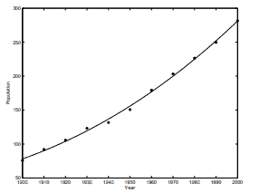
问题 4. We are given the following data for the total population of the United States, as determined by the
U. S. Census, for the years 1900 to \(2000 .\) The units are millions of people.
\begin{array}{cr}
t & y \\
\hline 1900 & 75.995 \\
1910 & 91.972 \\
1920 & 105.711 \\
1930 & 123.203 \\
1940 & 131.669 \\
1950 & 150.697 \\
1960 & 179.323 \\
1970 & 203.212 \\
1980 & 226.505 \\
1990 & 249.633 \\
2000 & 281.422 \\
\hline
\end{array}
Suppose we model the population growth by
$$
y \approx \beta_{1} t^{3}+\beta_{2} t^{2}+\beta_{3} t+\beta_{4}
$$
(a) Use normal equations for computing \(\beta\). Plot the resulting polynomial and the exact values \(\mathbf{y}\) in the same graph.
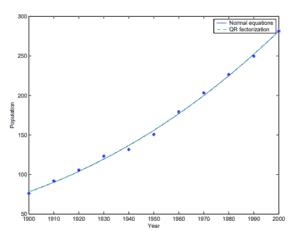
(b) Use the QR factorization to obtain \(\beta\) for the same problem. Plot the resulting polynomial and the exact values, as well as the polynomial in part (a), in the same graph. Also compare your coefficients with those obtained in part (a).
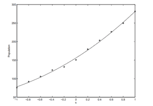
(c) Suppose we translate and scale the time variable \(t\) by
$$
s=(t-1950) / 50
$$
and use the model
$$
y \approx \beta_{1} s^{3}+\beta_{2} s^{2}+\beta_{3} s+\beta_{4}
$$
Now solve for the coefficients \(\beta\) and plot the polynomial and the exact values in the same graph. Which of the polynomials in part (a) through (c) gives the best fit to the data?
证明 . (a) The least squares problem is
$$
\min \|y-A \beta\|
$$
where
$$
A=\left[\begin{array}{cccc}
t_{1}^{3} & t_{1}^{2} & t_{1} & 1 \\
\vdots & & & \vdots \\
t_{n}^{3} & t_{n}^{2} & t_{n} & 1
\end{array}\right]
$$
\(n=11, t_{i}=1900+10(i-1) .\) We form the normal equations \(A^{T} A \beta=A^{T} y\) and solve for \(\beta\) to obtain
beta \(=\)
\(1.010415596011712 e-005\)
\(-4.961885780449666 \mathrm{e}-002\)
\(8.025770365215973 e+001\)
$$
-4.259196447217581 e+004
$$
The plot is shown in Figure 4 . Here we have \(\|y-A \beta\|_{2}=10.1\).
![]()
 (b)
Now we use the QR factorization to obtain beta2.
\(\gg[Q, R]=\mathrm{qr}(\mathrm{A}) ;\)
\(\gg \mathrm{b}=\) Q’*y;
\(\gg\) beta \(2=R(1: 4,1: 4) \backslash b(1: 4)\)
beta2 \(=\)
$$
\begin{array}{r}1.010353535409117 \mathrm{e}-005 \\ -4.961522727598729 \mathrm{e}-002 \\ 8.025062525889830 \mathrm{e}+001 \\ -4.258736497384948 \mathrm{e}+004\end{array}
$$
So \(\|\) beta \(2-\) beta \(\|_{2}=4.60 .\) The norm of the residual is essentially the same as in part (a), with a difference of \(1.08 \times 10^{-10}\). This shows the least-squares problem is very ill-conditioned, since a small change in the residual yields a relatively large change in the solution vector. However, Figure 5 shows that the two fits are hardly distinguishable on a graph (mostly because the residuals are both small).
(b)
Now we use the QR factorization to obtain beta2.
\(\gg[Q, R]=\mathrm{qr}(\mathrm{A}) ;\)
\(\gg \mathrm{b}=\) Q’*y;
\(\gg\) beta \(2=R(1: 4,1: 4) \backslash b(1: 4)\)
beta2 \(=\)
$$
\begin{array}{r}1.010353535409117 \mathrm{e}-005 \\ -4.961522727598729 \mathrm{e}-002 \\ 8.025062525889830 \mathrm{e}+001 \\ -4.258736497384948 \mathrm{e}+004\end{array}
$$
So \(\|\) beta \(2-\) beta \(\|_{2}=4.60 .\) The norm of the residual is essentially the same as in part (a), with a difference of \(1.08 \times 10^{-10}\). This shows the least-squares problem is very ill-conditioned, since a small change in the residual yields a relatively large change in the solution vector. However, Figure 5 shows that the two fits are hardly distinguishable on a graph (mostly because the residuals are both small).
![]()
 (c) We now perform a change of the independent variable
$$
s=(t-1950) / 50
$$
so that \(s \in[-1,1] .\) We again set up the least square system and solve:
\(\gg[Q, R]=q r(A)\)
\(\gg b=Q^{\prime} * b ;\)
\(\gg b=Q^{\prime} * y ;\)
\(\gg\) beta \(3=R(1: 4,1: 4) \backslash b(1: 4) ;\)
\(\gg\) betas
beta3 \(=\)
$$
\begin{array}{r}1.262941919191900 \mathrm{e}+000 \\ 2.372613636363639 \mathrm{e}+001 \\ 1.003659217171717 \mathrm{e}+002 \\ 1.559042727272727 \mathrm{e}+002\end{array}
$$
Note that the coefficients are different because we are using a different basis. The residual is again essentially the same as parts (a) and (b) (the difference is \(1.54 \times 10^{-11}\) ). So even though the coefficients are quite different, the quality of the fit is essentially the same (even though (c) is more accurate by just a tiny bit).
(c) We now perform a change of the independent variable
$$
s=(t-1950) / 50
$$
so that \(s \in[-1,1] .\) We again set up the least square system and solve:
\(\gg[Q, R]=q r(A)\)
\(\gg b=Q^{\prime} * b ;\)
\(\gg b=Q^{\prime} * y ;\)
\(\gg\) beta \(3=R(1: 4,1: 4) \backslash b(1: 4) ;\)
\(\gg\) betas
beta3 \(=\)
$$
\begin{array}{r}1.262941919191900 \mathrm{e}+000 \\ 2.372613636363639 \mathrm{e}+001 \\ 1.003659217171717 \mathrm{e}+002 \\ 1.559042727272727 \mathrm{e}+002\end{array}
$$
Note that the coefficients are different because we are using a different basis. The residual is again essentially the same as parts (a) and (b) (the difference is \(1.54 \times 10^{-11}\) ). So even though the coefficients are quite different, the quality of the fit is essentially the same (even though (c) is more accurate by just a tiny bit).
![]()
更多线性代数代写案例请参阅此处。
(b)
Now we use the QR factorization to obtain beta2.
\(\gg[Q, R]=\mathrm{qr}(\mathrm{A}) ;\)
\(\gg \mathrm{b}=\) Q’*y;
\(\gg\) beta \(2=R(1: 4,1: 4) \backslash b(1: 4)\)
beta2 \(=\)
$$
\begin{array}{r}1.010353535409117 \mathrm{e}-005 \\ -4.961522727598729 \mathrm{e}-002 \\ 8.025062525889830 \mathrm{e}+001 \\ -4.258736497384948 \mathrm{e}+004\end{array}
$$
So \(\|\) beta \(2-\) beta \(\|_{2}=4.60 .\) The norm of the residual is essentially the same as in part (a), with a difference of \(1.08 \times 10^{-10}\). This shows the least-squares problem is very ill-conditioned, since a small change in the residual yields a relatively large change in the solution vector. However, Figure 5 shows that the two fits are hardly distinguishable on a graph (mostly because the residuals are both small).
(c) We now perform a change of the independent variable
$$
s=(t-1950) / 50
$$
so that \(s \in[-1,1] .\) We again set up the least square system and solve:
\(\gg[Q, R]=q r(A)\)
\(\gg b=Q^{\prime} * b ;\)
\(\gg b=Q^{\prime} * y ;\)
\(\gg\) beta \(3=R(1: 4,1: 4) \backslash b(1: 4) ;\)
\(\gg\) betas
beta3 \(=\)
$$
\begin{array}{r}1.262941919191900 \mathrm{e}+000 \\ 2.372613636363639 \mathrm{e}+001 \\ 1.003659217171717 \mathrm{e}+002 \\ 1.559042727272727 \mathrm{e}+002\end{array}
$$
Note that the coefficients are different because we are using a different basis. The residual is again essentially the same as parts (a) and (b) (the difference is \(1.54 \times 10^{-11}\) ). So even though the coefficients are quite different, the quality of the fit is essentially the same (even though (c) is more accurate by just a tiny bit).

E-mail: [email protected] 微信:shuxuejun
uprivate™是一个服务全球中国留学生的专业代写公司 专注提供稳定可靠的北美、澳洲、英国代写服务 专注于数学,统计,金融,经济,计算机科学,物理的作业代写服务
[…] Arnold在20世纪七十年代就说过,二十一世纪的数学将会是线性代数和组合的世纪,不是代数几何的世纪。这句话虽然不算太准确,但是线性代数和组合的技巧确实变得非常重要。所以学好线性代数将会对于以后的数学研究有极大的帮助,如果有看这个帖子的人以后会做数学研究的话。 我们最近接过的比较难的线性代数的单子是一个德语的单子,是Humboldt-Universität zu Berlin的德语的Advancd linear algebra,实际上是advance spectral theorey,总之线性代数难起来是可以非常难的。因为线性代数是很多后续课程的核心技巧部分。 这一次的是Math 4570这门课的一份代写答案,前两次次作业客户自己做了,到第三次才找到我们,当时前两次分数惨不忍睹,要想拿到好成绩后续作业必须尽量满分然后考试考高,但是这个客户的考试条件对于我们协助考试相当不利,出于我们的努力,最后还是勉强实现了客户想要成绩在90以上的目标。类似的案例还有这个 Problem 1. 1. Let (V) and (W) be vector spaces over a field (F). Let (0_{mathrm{V}}) and (0_{mathrm{W}}) be the zero vectors of (V) and (W) respectively. Let (T: V rightarrow W) be a function. Prove the following. (a) If (T) is a linear transformation, then (Tleft(0_{V}right)=0_{mathrm{W}}). (b) (T) is a linear transformation if and only if $$ T(alpha x+beta y)=alpha T(x)+beta T(y) $$ for all (x, y in V) and (alpha, beta in F). (c) (T) is a linear transformation if and only if $$ Tleft(sum_{i=1}^{n} alpha_{i} x_{i}right)=sum_{i=1}^{n} alpha_{i} Tleft(x_{i}right) $$ for all (x_{1}, ldots, x_{n} in V) and (alpha_{1}, ldots, alpha_{n} in F) Proof . (a) We have that (Tleft(O_{v}right)=Tleft(O_{v}+U_{v}right)=Tleft(O_{v}right)+Tleft(0_{v}right)). Adding (-Tleft(0_{v}right)) to both sider we get (-underbrace{Tleft(0_{v}right)+Tleft(0_{v}right)}_{O_{w}}=-underbrace{Tleft(0_{v}right)+Tleft(0_{v}right)}_{O_{w}}+Tleft(0_{v}right)) So, (quad O_{W}=Tleft(U_{v}right)) (b) This follows from (c) with (n=2), (c) (Rightarrow) Suppose (T) is linear. We prove the resvit by induction, If (n=1), then (Tleft(alpha_{1} x_{1}right)=alpha_{1} Tleft(x_{1}right)) since (T) is linear. If (n=2), Then (Tleft(x_{1} x_{1}+alpha_{2} x_{2}right)=Tleft(alpha_{1} x_{1}right)+Tleft(alpha_{2} x_{2}right)) (=alpha_{1} Tleft(x_{1}right)+alpha_{2} Tleft(x_{2}right)), Let (k geqslant 2) in formula. Suppose the formula is true for (n=k), Then $$ Tleft(alpha_{1} x_{1}+alpha_{2} x_{2}+ldots+alpha_{k} x_{k}+alpha_{k+1} x_{k+1}right)=Tleft(alpha_{1} x_{1}+ldots+alpha_{k} x_{k}right)+Tleft(alpha_{k+1} x_{k+1}right)=…$$ $$=alpha_{1} Tleft(x_{1}right)+alpha_{2} Tleft(x_{2}right)+alpha_{k} Tleft(x_{k}right)+alpha_{k+1} Tleft(x_{k+1}right)$$ ((Leftarrow)) Suppose (Tleft(sum_{i=1}^{n} alpha_{i} x_{i}right)=sum_{i=1}^{n} alpha_{i} Tleft(x_{i}right)) for all (alpha_{i} in F) and (x_{i} in V_{1}) Setting (n=2) and (alpha_{1}=alpha_{2}=1) we get (Tleft(x_{1}+x_{2}right)=Tleft(x_{1}right)+Tleft(x_{2}right)) for all (x_{1}, x_{2} in V). Setting (n=1), we get (Tleft(alpha_{1} x_{1}right)=alpha_{1} Tleft(x_{1}right)) for all (alpha_{1} in F) and (x_{1} in V), Thus, (T) is linear, Problem 2. Verify whether or not (T: V rightarrow W) is a linear transformation. If (T) is a linear transformation then: (i) compute the nullspace of (T,) (ii) compute the range of (T,) (iii) compute the nullity of (T,) (iv) compute the rank of (T,) (v) determine if (T) one-to-one, and (vi) determine if (T) is onto. (a) (T: mathbb{R}^{3} rightarrow mathbb{R}^{2}) given by (T(a, b, c)=(a-b, 2 c)) (b) (T: mathbb{R}^{2} rightarrow mathbb{R}^{2}) given by (T(a, b)=left(a-b, b^{2}right)) (c) (T: M_{2,3}(mathbb{R}) rightarrow M_{2,2}(mathbb{R})) given by $$ Tleft(begin{array}{lll} a & b & c \ d & e & f end{array}right)=left(begin{array}{cc} 2 a-b & c+2 d \ 0 & 0 end{array}right) $$ (d) (T: P_{2}(mathbb{R}) rightarrow P_{3}(mathbb{R})) given by (Tleft(a+b x+c x^{2}right)=a+b x^{3}) (e) (T: P_{2}(mathbb{R}) rightarrow P_{2}(mathbb{R})) given by (Tleft(a+b x+c x^{2}right)=(1+a)+(1+b) x+(1+c) x^{2}) Proof . (a)This linear, Let (x=(a, b, c)) and (y=(d, e, f)), Let (alpha, beta in mathbb{R}), Then (begin{aligned} T(alpha x+beta y) &=T(alpha a+beta d, alpha b+beta e, alpha c+beta f) \ &=(alpha a+beta d-alpha b-beta e, 2 alpha c+2 beta f) \ &=(alpha a-alpha b, 2 alpha c)+(beta d-beta e, 2 beta f) \ &=alpha(a-b, 2 c)+beta(d-e, 2 f) \ &=alpha T(x)+beta T(y) . end{aligned}) (i)(ii) are easy to check, (iii) A basis for (N(T)) is (left{left(begin{array}{l}1 \ 0end{array}right)right} .) So, Nullity ((T)=1). (iv) (R(T)=mathbb{R}^{2}), So, (operatorname{rank}(T)=2), (v) (T) is not one-to one. For example, (T(0,0,0)=T(1,1,0)=(0,0)) (vi) T is onto since (R(t)=mathbb{R}^{2}). (b) T is not linear, For example, (T(1,1)+T(2,2)=left(1-1,1^{2}right)+left(2-2,2^{2}right)) (=(0,1)+(0,4)=(0,5)) but (T((1,1)+(2,2))=T(3,3)=left(3-3,3^{2}right)=(0,9)) (c) (T) is linear. Let (x=left(begin{array}{lll}a_{1} & b_{1} & c_{1} \ d_{1} & e_{1} & f_{1}end{array}right)) and (y=left(begin{array}{ll}a_{2} & b_{2} c_{2} \ d_{2} & e_{2} f_{2}end{array}right)) and (alpha, beta in mathbb{R},) Then (begin{aligned} &T(alpha x+beta y)=Tleft(begin{array}{cc}alpha a_{1}+beta a_{2} & alpha b_{1}+beta b_{2} & alpha c_{1}+p_{2} z_{2} \ alpha d_{1}+beta d_{2} & alpha e_{1}+beta e_{2} & alpha f_{1}+beta f_{2}end{array}right) \ &=left(begin{array}{cc}2left(alpha a_{1}+beta a_{2}right)-left(alpha_{1}+beta b_{2}right) & alpha c_{1}+beta c_{2}+2left(alpha d_{1}+beta d_{2}right) \ 0 & 0end{array}right) \ &=alphaleft(begin{array}{cc}2 a_{1}-b_{1} & c_{1}+2 d_{1} \ 0 & 0end{array}right)+betaleft(begin{array}{cc}2 a_{2}-b_{2} & c_{2}+2 d_{2} \ 0 & 0end{array}right) \ &=alpha T(x)+beta T(y) end{aligned}) Problem 3. Let (a) and (b) be real numbers where (a<b). Let (C(mathbb{R})) be the vector space of continuous functions on the real line as in HW # 1. Let (T: C(mathbb{R}) rightarrow mathbb{R}) given by $$ T(f)=int_{a}^{b} f(t) d t $$ Verify whether or not (T) is linear. Proof . Let (alpha, beta in mathbb{R}) and (f, g in C(mathbb{R})). Then (begin{aligned} T(alpha f+beta g)=int_{a}^{b} alpha f(t)+beta g(t) d t &=alpha int_{a}^{b} f(t) d t+beta int_{a}^{b} g(x) d t \ &=alpha T(f)+beta T(g) end{aligned}) Problem 4. Let (F) be a field. Recall that if (A in M_{m, n}(F)) then we can make a linear transformation (L_{A}: F^{n} rightarrow F^{m}) where (L_{A}(x)=A x) is left-sided matrix multiplication. In each problem, calculate (L_{A}(x)) for the given (A) and (x) (a) (F=mathbb{R}, L_{A}: mathbb{R}^{2} rightarrow mathbb{R}^{2}, A=left(begin{array}{cc}1 & pi \ frac{1}{2} & -10end{array}right), x=left(begin{array}{c}17 \ -5end{array}right)) (b) (F=mathbb{C}, L_{A}: mathbb{C}^{3} rightarrow mathbb{C}^{2}, A=left(begin{array}{ccc}-i & 1 & 0 \ 1+i & 0 & -1end{array}right), x=left(begin{array}{c}-2 i \ 4 \ 1.57end{array}right)) Proof . (a) (L_{A}(x)=left(begin{array}{cc}1 & pi \ y / 2 & -10end{array}right)left(begin{array}{c}17 \ -5end{array}right)=left(begin{array}{cc}17 & -5 pi \ frac{17}{2} & +50end{array}right)=left(begin{array}{c}17-5 pi \ 117 / 2end{array}right)) (b) (L_{A}(x)=left(begin{array}{ccc}-i & 1 & 0 \ 1+i & 0 & -1end{array}right)left(begin{array}{c}-2 i \ 4 \ 1,57end{array}right)=left(begin{array}{c}2 i^{2}+4+0 \ -2 i-2 i^{2}+0-1,57end{array}right)) (=left(begin{array}{c}2 \ -2 i+0.43end{array}right)) Problem 5. 5. Let (V) and (W) be vector spaces over a field (F). Let (T: V rightarrow W) be a linear transformation. Let (v_{1}, ldots, v_{n} in V) such that (operatorname{span}left(left{v_{1}, ldots, v_{n}right}right)=V), then (operatorname{span}left(left{Tleft(v_{1}right), ldots, Tleft(v_{n}right)right}right)=R(T)). Proof . Let (y in R(T)). Then there exists (x in V) with (T(x)=y) by def of (R(T)). Since (x in V) and (V=operatorname{span}left(left{v_{1}, ldot
s, v_{n}right}right)) we have (x=c_{1} v_{1}+c_{2} v_{2} t_{14}+c_{1} v_{1}) for some (c_{i} in F), So, (y=T(x)=Tleft(c_{1} v_{1}+c_{2} v_{2}+u_{1}+c_{1} v_{n}right)=c_{1} Tleft(v_{1}right)+c_{2} Tleft(v_{2}right)+m+c_{n} Tleft(v_{n}right)) co (y in operatorname{span}left(left{Tleft(v_{1}right), Tleft(v_{2}right), ldots, Tleft(v_{n}right)right}right)) Hence (R(T) subseteq operatorname{span}left(left{Tleft(v_{1}right), Tleft(v_{2}right)_{1}, ldots, Tleft(v_{n}right)right}right)) Thus, (left.R(T)=operatorname{spn}left(left{Tleft(V_{1}right)_{1}, mu_{1}right) Tleft(V_{n}right)right}right)=R(T)) Problem 6. 6. Let (V) and (W) be vector spaces over a field (F). Let (T: V rightarrow W) be a linear transformation. Let (0_{mathrm{V}}) and (0_{mathrm{W}}) be the zero vectors of (V) and (W) respectively. (a) Prove that (T) is one-to-one if and only if (N(T)=left{0_{mathrm{V}}right}). (b) Suppose that (V) and (W) are both finite-dimensional and (operatorname{dim}(V)=) (operatorname{dim}(W)). Prove that (T) is one-to-one if and only if (T) is onto. (c) Suppose that (V) and (W) are both finite-dimensional. Prove that if (T) is one-to-one and onto then (operatorname{dim}(V)=operatorname{dim}(W)) Proof . (Rightarrow) is easy. Suppuse that T is one-to-one. We know that (Tleft(0_{v}right)=0_{w}) So, (O_{v} in N(T)). Since (T) is one-to-one, (0_{V}) is the only solution Thus, (N(T)={x in V mid T(x)=0 w}=left{0_{v}right}) Let (x, y in V) with (T(x)=T(y)) Then (T(x)-T(y)=0 w). So, (T(x-y)=O_{w}), since (T) ir linear. Thus, (x-y in N(T)). so, (x-y=0_{V}). Thus, (x=y). (b) Suppoce that (operatorname{dim}(V)=operatorname{dim}(W)) Rocale that nullity ((T)+operatorname{can} k(T)=operatorname{dim}(V)) (Rightarrow) Suppore that (T) is one-tu-one. By pact ((a)), (N(T)={0,}}) so nullity ((T)=0), So, mea (0+operatorname{cank}(T)=operatorname{dim}(V)) Since (operatorname{dim}(V)=operatorname{dim}(omega)) we get 1. Since (R) (T) is a subspace of w and since dim (R(T) Hence T is onto. (Leftrightarrow) Suppose that (T) is onto. So, (R(T)=W), So, (R(T)=W_{C}=operatorname{dim}(w)), Thus, rank ((T)=operatorname{dim}(v)) since (dim(w)=dim(v))we get that (null(T)+dim(T)=dim(v)) because (null(T)+dim(w)=dim(w)), so (null(T)=0), thus (N(T)={0_v}). (c) Supeose that (V) and (W) ane finite dimen ritinal cand T is (1-1) and onto. basis for (V), Let (w_{i}=Tleft(v_{i}right)) for (i=1,2, ldots, n), By thm in the notes since (T) By thm in the notes (left.w_{1}, w_{2}, ldots, w_{n}right}) is a basis fur (w_{1}) s a basis ((V)=n=operatorname{dim}(omega)), Problem 7. 7. Let (V) and (W) be finite dimensional vector spaces and let (T: V rightarrow W) be a linear transformation. (a) If (operatorname{dim}(V)<operatorname{dim}(W),) then (T) is not onto. (b) If (operatorname{dim}(V)>operatorname{dim}(W),) then (T) is not one-to-one. Proof . (a) is easy. (b) We have that (nullity (T)+rank(T)=operatorname{dim}(V)). Since (operatorname{din}(V)>operatorname{dim}(omega)) we have that $$nullity ((T)+ranK(T)>operatorname{dim}(W)$$ if (nullity(T)=0), then (rank(T)>dim(W)). But that would imply that (R(T)), which is a subspace of (W) but has bigger dimension than (W)), this couyld not happen, so (nullity (T) >0), So, (operatorname{dim}(N(T))>0). so (N(T) neqleft{0_{v}right})so, (T) is not one to one b problem 6. 更多线性代数代写案例请参阅此处。 […]