统计代写| URecap stat代写
统计代考
4.10 Recap
The expectation of a discrete r.v. $X$ is
$$
E(X)=\sum_{x} x P(X=x) \text {. }
$$
An equivalent “ungrouped” way of calculating expectation is
$$
E(X)=\sum_{s} X(s) P({s})
$$
where the sum is taken over pebbles in the sample space. Expectation is a single number summarizing the center of mass of a distribution. A single-number summary of the spread of a distribution is the variance, defined by
$$
\operatorname{Var}(X)=E(X-E X)^{2}=E\left(X^{2}\right)-(E X)^{2} .
$$
The square root of the variance is called the standard deviation.
190
Expectation is linear:
$$
E(c X)=c E(X) \text { and } E(X+Y)=E(X)+E(Y),
$$
regardless of whether $X$ and $Y$ are independent or not. Variance is not linear:
$$
\operatorname{Var}(c X)=c^{2} \operatorname{Var}(X)
$$
and
$$
\operatorname{Var}(X+Y) \neq \operatorname{Var}(X)+\operatorname{Var}(Y)
$$
in general (an important exception is when $X$ and $Y$ are independent). A very important strategy for calculating the expectation of a discrete ruv. $X$ is to tal bridge. This technique is especially powerful because the indicator r.v.s need not be independent; linearity holds even for dependent r.v.s. The strategy can be summarized in the following three steps.
- Represent the r.v. $X$ as a sum of indicator r.v.s. To decide how to define the indicators, think about what $X$ is counting. For example, if $X$ is the number of local maxima, as in the Putnam problem, then we should create an indicator for each local maximum that could occur.
- Use the fundamental bridge to calculate the expected value of each indicator. When applicable, symmetry may be very helpful at this stage.
- By linearity of expectation, $E(X)$ can be obtained by adding up the expectations of the indicators.
Another tool for computing expectations is LOTUS, which says we can calculate the expectation of $g(X)$ using only the PMF of $X$, via
$$
E(g(X))=\sum_{x} g(x) P(X=x) .
$$
If $g$ is non-linear, it is a grave mistake to attempt to calculate $E(g(X))$ by swapping the $E$ and the $g$.
Four new discrete distributions to add to our list are the Geometric, Negative Binomial, Negative Hypergeometric, and Poisson distributions. A Geom $(p)$ r.v. is the number of failures before the first success in a sequence of independent Bernoulli trials with probability $p$ of success, and an NBin $(r, p) r, v$, is the number of failures mial except, in terms of drawing balls from an urn, the Negative Hypergeometric samples without replacement and the Negative Binomial samples with replacement. (We also introduced the First Success distribution, which is just a Geometric shifted so that the success is included.)
A Poisson $r . v .$ is often used as an approximation for the number of successes that
Expectation
191 occur when there are many independent or weakly dependent trials, where each trial has a small probability of success. In the Binomial story, all the trials have the same probability $p$ of success, but in the Poisson approximation, different trials can have different (but small) probabilities $p_{j}$ of success.
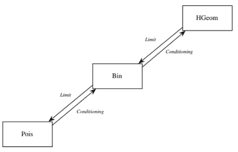
The Poisson, Binomial, and Hypergeometric distributions are mutually connected via the operations of conditioning and taking limits, as illustrated in Figure $4.8$. In the rest of this book, we’ll continue to introduce new named distributions and add them to this family tree, until everything is connected!
统计代考
4
4.10 回顾
离散 r.v. 的期望$X$ 是
$$
E(X)=\sum_{x} x P(X=x) \text {。 }
$$
计算期望的等效“未分组”方式是
$$
E(X)=\sum_{s} X(s) P({s})
$$
其中总和取自样本空间中的鹅卵石。期望是总结分布的质心的单个数字。分布分布的单个数字摘要是方差,定义为
$$
\operatorname{Var}(X)=E(X-E X)^{2}=E\left(X^{2}\right)-(E X)^{2} 。
$$
方差的平方根称为标准差。
190
期望是线性的:
$$
E(c X)=c E(X) \text { 和 } E(X+Y)=E(X)+E(Y),
$$
不管 $X$ 和 $Y$ 是否独立。方差不是线性的:
$$
\operatorname{Var}(c X)=c^{2} \operatorname{Var}(X)
$$
和
$$
\operatorname{Var}(X+Y) \neq \operatorname{Var}(X)+\operatorname{Var}(Y)
$$
一般来说(一个重要的例外是当 $X$ 和 $Y$ 是独立的)。计算离散 ruv 期望的一个非常重要的策略。 $X$ 是 tal 桥。这种技术特别强大,因为指标 r.v.s 不需要是独立的;线性甚至适用于相关的 r.v.s.该策略可以概括为以下三个步骤。
- 代表房车$X$ 作为指标 r.v.s 的总和。要决定如何定义指标,请考虑 $X$ 的计数。例如,如果 $X$ 是局部最大值的数量,如 Putnam 问题,那么我们应该为每个可能出现的局部最大值创建一个指标。
- 使用基础桥计算每个指标的期望值。在适用的情况下,对称性在此阶段可能非常有用。
3、通过期望的线性,可以将指标的期望相加得到$E(X)$。
另一个计算期望值的工具是 LOTUS,它说我们可以仅使用 $X$ 的 PMF 来计算 $g(X)$ 的期望值,通过
$$
E(g(X))=\sum_{x} g(x) P(X=x) 。
$$
如果$g$ 是非线性的,那么试图通过交换$E$ 和$g$ 来计算$E(g(X))$ 是一个严重的错误。
添加到我们列表中的四个新离散分布是几何分布、负二项分布、负超几何分布和泊松分布。 Geom $(p)$ r.v.是在成功概率为 $p$ 的独立伯努利试验序列中第一次成功之前的失败次数,并且 NBin $(r, p) r, v$, 是失败的次数 mial 除了在绘图方面瓮中的球,没有替换的负超几何样本和有替换的负二项式样本。 (我们还介绍了 First Success 分布,它只是一个几何偏移,因此包含了成功。)
泊松 $r 。 v .$ 通常用作成功次数的近似值
期待
当有许多独立的或弱依赖的试验时,会发生 191,其中每个试验的成功概率很小。在二项式故事中,所有试验都有相同的成功概率 $p$,但在泊松近似中,不同的试验可以有不同(但很小)的成功概率 $p_{j}$。
泊松分布、二项分布和超几何分布通过调节和取极限的操作相互连接,如图 $4.8$ 所示。在本书的其余部分,我们将继续介绍新的命名分布并将它们添加到这个家谱中,直到一切都连接起来!
。
R语言代写

统计代写|SAMPLE SPACES AND PEBBLE WORLD stat 代写 请认准UprivateTA™. UprivateTA™为您的留学生涯保驾护航。