统计代写| Metropolis-Hastings stat代写
统计代考
$12.4 \quad R$
Metropolis-Hastings
Here’s how to implement the Metropolis-Hastings algorithm for Example 12.1.8, the Normal-Normal model. First, we choose our observed value of $Y$ and decide on values for the constants $\sigma, \mu$, and $\tau$ :
$\mathrm{y}<-3$
sigma $<-1$
$\mathrm{mu}<-0$
We also need to choose the standard deviation of the proposals for step 1 of the algorithm, as explained in Example 12.1.8; for this problem, we let $d=1$. We set the number of iterations to run, and we allocate a vector theta of length $10^{4}$ which we will fill with our simulated draws:
$d<-1$
niter $<-10^{-4}$
theta <- rep (0, niter)
Now for the main loop. We initialize $\theta$ to the observed value $y$, then run the algorithm described in Example 12.1.8:
theta [1] <- $\mathrm{y}$
for ( $i$ in $2:$ niter) {
theta.p <- theta[i-1] + rnorm $(1,0, d)$
$r<-\operatorname{dnorm}(y$, theta.p,sigma) * dnorm(theta.p, mu, tau) / (dnorm (y, theta[i-1], sigma) * dnorm(theta[i-1], mu, tau))
$f l i p<-r b i n o m(1,1, \min (r, 1))$
theta $[i]<-$ if $(f l i p=1)$ theta.p else theta $[i-1]$
Let’s step through each line inside the loop. The proposed value of $\theta$ is theta.p, which equals the previous value of $\theta$ plus a Normal random variable with mean 0 and standard deviation d (recall that rnorm takes the standard deviation and not the variance as input). The ratio $r$ is
$$
\frac{f_{\theta \mid Y}\left(x^{\prime} \mid y\right)}{f_{\theta \mid Y}(x \mid y)}=\frac{e^{-\frac{1}{2 \sigma^{2}}\left(y-x^{\prime}\right)^{2}} e^{-\frac{1}{2 T^{2}}\left(x^{\prime}-\mu\right)^{2}}}{e^{-\frac{1}{2 \sigma^{2}}(y-x)^{2}} e^{-\frac{1}{2 T^{2}}(x-\mu)^{2}}}
$$
where theta.p is playing the role of $x^{\prime}$ and theta [i-1] is playing the role of $x$. The coin flip to determine whether to accept or reject the proposal is flip, which is a coin flip with probability min $(r, 1)$ of Heads (encoding Heads as 1 and Tails as 0). Finally, we set theta[i] equal to the proposed value if the coin flip lands Heads, and keep it at the previous value otherwise.
556
The vector theta now contains all of our simulation draws. We typically discard some of the initial draws to give the chain some time to approach the stationary distribution. The following line of code discards the first half of the draws:
theta <- theta [- (1: (niter/2))]
To see what the remaining draws look like, we can create a histogram using hist (theta). We can also compute summary statistics such as mean(theta) and var (theta), which give us the sample mean and sample variance.
Gibbs
Now let’s implement Gibbs sampling for Example 12.2.6, the chicken-egg story with unknown hatching probability and invisible unhatched eggs. The first step is to decide on our observed value of $X$, as well as the constants $\lambda, a, b$ :
$x<-7$
lambda <- 10
$a<-1$ $b<-1$
Next we decide how many iterations to run, and we allocate space for our results, creating two vectors $\mathrm{p}$ and $\mathrm{N}$ of length $10^{4}$ which we will fill with our simulated draws:
niter $<-10^{-4}$
$p<-\operatorname{rep}(0$, niter $)$ $N<-\operatorname{rep}(0$, niter $)$
Finally, we’re ready to run the Gibbs sampler. We initialize $p$ and $N$ to the values
$0.5$ and $2 x$, respectively, and then we run the algorithm as explained in Example
$12.2 .6$ :
统计代考
$ 12.4 \四R $
大都会-黑斯廷斯
下面是如何实现例 12.1.8 的 Metropolis-Hastings 算法,即 Normal-Normal 模型。首先,我们选择我们观察到的 $Y$ 值并确定常量 $\sigma、\mu$ 和 $\tau$ 的值:
$\mathrm{y}<-3$
西格玛 $<-1$
$\mathrm{mu}<-0$
我们还需要为算法的第 1 步选择建议的标准差,如示例 12.1.8 中所述;对于这个问题,我们让$d=1$。我们设置要运行的迭代次数,并分配一个长度为 $10^{4}$ 的向量 theta,我们将用模拟绘图填充它:
$d<-1$
硝石 $<-10^{-4}$
theta <- rep (0, niter)
现在是主循环。我们将 $\theta$ 初始化为观测值 $y$,然后运行示例 12.1.8 中描述的算法:
theta [1] <- $\mathrm{y}$
for ($i$ in $2:$ niter) {
theta.p <- theta[i-1] + rnorm $(1,0, d)$
$r<-\operatorname{dnorm}(y$, theta.p,sigma) * dnorm(theta.p, mu, tau) / (dnorm (y, theta[i-1], sigma) * dnorm(theta[ i-1], mu, tau))
$f l i p<-r b i n o m(1,1, \min (r, 1))$
theta $[i]<-$ if $(f l i p=1)$ theta.p else theta $[i-1]$
让我们逐步浏览循环内的每一行。 $\theta$ 的建议值为 theta.p,它等于 $\theta$ 的先前值加上平均值为 0 和标准差为 d 的正态随机变量(请记住,rnorm 将标准差而不是方差作为输入) .比率 $r$ 是
$$
\frac{f_{\theta \mid Y}\left(x^{\prime} \mid y\right)}{f_{\theta \mid Y}(x \mid y)}=\frac{e^{ -\frac{1}{2 \sigma^{2}}\left(yx^{\prime}\right)^{2}} e^{-\frac{1}{2 T^{2}}\左(x^{\prime}-\mu\right)^{2}}}{e^{-\frac{1}{2 \sigma^{2}}(yx)^{2}} e^{ -\frac{1}{2 T^{2}}(x-\mu)^{2}}}
$$
其中 theta.p 扮演 $x^{\prime}$ 的角色,而 theta [i-1] 扮演 $x$ 的角色。决定接受还是拒绝提议的掷硬币是翻转,这是一个正面概率为 min $(r, 1)$ 的硬币翻转(将 Heads 编码为 1,Tails 编码为 0)。最后,如果掷硬币正面朝上,我们将 theta[i] 设置为等于建议的值,否则将其保持在先前的值。
556
向量 theta 现在包含我们所有的模拟绘图。我们通常会丢弃一些初始抽签,以便给链一些时间来接近平稳分布。以下代码行丢弃了前半部分的绘制:
theta <- theta [- (1: (niter/2))]
要查看剩余的绘图是什么样子,我们可以使用 hist (theta) 创建一个直方图。我们还可以计算汇总统计数据,例如 mean(theta) 和 var (theta),它们为我们提供了样本均值和样本方差。
吉布斯
现在让我们为示例 12.2.6 实施 Gibbs 抽样,这是一个孵化概率未知且未孵化的鸡蛋不可见的鸡蛋故事。第一步是确定我们观察到的 $X$ 值,以及常数 $\lambda, a, b$ :
$x<-7$
λ <- 10
$a<-1$ $b<-1$
接下来我们决定要运行多少次迭代,并为我们的结果分配空间,创建两个向量 $\mathrm{p}$ 和 $\mathrm{N}$,长度为 $10^{4}$,我们将用我们的模拟填充绘制:
硝石 $<-10^{-4}$
$p<-\operatorname{rep}(0$, niter $)$ $N<-\operatorname{rep}(0$, niter $)$
最后,我们准备运行 Gibbs 采样器。我们将 $p$ 和 $N$ 初始化为值
$0.5$ 和 $2 x$,然后我们按照示例中的说明运行算法
12.2 .6 美元:

统计代写|SAMPLE SPACES AND PEBBLE WORLD stat 代写 请认准UprivateTA™. UprivateTA™为您的留学生涯保驾护航。