运筹学(Operation)是近代应用数学的一个分支。它把具体的问题进行数学抽象,然后用像是统计学、数学模型和算法等方法加以解决,以此来寻找复杂问题中的最佳或近似最佳的解答。
作为专业的留学生服务机构,Assignmentexpert™多年来已为美国、英国、加拿大、澳洲等留学热门地的学生提供专业的学术服务,包括但不限于论文代写,A作业代写,Dissertation代写,Report代写,Paper代写,Presentation代写,网课代修等等。为涵盖高中,本科,研究生等海外留学生提供辅导服务,辅导学科包括数学,物理,统计,化学,金融,经济学,会计学等全球99%专业科目。写作团队既有专业英语母语作者,也有海外名校硕博留学生,每位写作老师都拥有过硬的语言能力,专业的学科背景和学术写作经验。我们承诺100%原创,100%专业,100%准时,100%满意。
my-assignmentexpert愿做同学们坚强的后盾,助同学们顺利完成学业,同学们如果在学业上遇到任何问题,请联系my-assignmentexpert™,我们随时为您服务!
运筹学代写
Our development to this point, including the above proof of the fundamental theorem, has been based only on elementary properties of systems of linear equations. These results, however, have interesting interpretations in terms of the theory of convex sets that can lead not only to an alternative derivation of the The main link between the algebraic and geometric theories is the formal relation between basic feasible solutions of linear inequalities in standard form and extreme points of polytopes. We establish this correspondence as follows. The reader is referred to Appendix B for a more complete summary of concepts related to convexity, but the definition of an extreme point is stated here.
Definition A point $\mathbf{x}$ in a convex set $C$ is said to be an extreme point of $C$ if there are no two distinct points $\mathbf{x}{1}$ and $\mathbf{x}{2}$ in $C$ such that $\mathbf{x}=\alpha \mathbf{x}{1}+(1-\alpha) \mathbf{x}{2}$ for some $\alpha, 0<\alpha<1$.
$2.5$ Relations to Convex Geometry
29
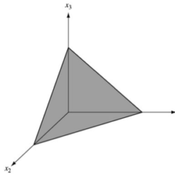
An extreme point is thus a point that does not lie strictly within a line segment connecting two other points of the set. The extreme points of a triangle, for example, are its three vertices.
Theorem (Equivalence of Extreme Points and Basic Solutions) Let $\mathbf{A}$ be an $m \times n$ matrix of rank $m$ and $\mathbf{b}$ an $m$-vector. Let $K$ be the convex polytope consisting of all $n$-vectors $\mathbf{x}$ satisfying
$(2.19)$
A vector $\mathbf{x}$ is an extreme point of $K$ if and only if $\mathbf{x}$ is a basic feasible solution to $(2,19)$.
Proof Suppose first that $\mathbf{x}=\left(x_{1}, x_{2}, \ldots, x_{m}, 0,0, \ldots, 0\right)$ is a basic feasible solution to $(2.19)$. Then
$$
x_{1} \mathbf{a}{1}+x{2} \mathbf{a}{2}+\cdots+x{m} \mathbf{a}{m}=\mathbf{b} $$ where $\mathbf{a}{1}, \mathbf{a}{2}, \ldots, \mathbf{a}{m}$, the first $m$ columns of $\mathbf{A}$, are linearly independent. Suppose that $\mathbf{x}$ could be expressed as a convex combination of two other points in $K$; say, $\mathbf{x}=\alpha \mathbf{y}+(1-\alpha) \mathbf{z}, 0<\alpha<1, \mathbf{y} \neq \mathbf{z}$. Since all components of $\mathbf{x}, \mathbf{y}, \mathbf{z}$ are nonnegative and since $0<\alpha<1$, it follows immediately components of $\mathbf{y}$ and $\mathbf{z}$ are zero. Thus, in particular, we have
$$
y_{1} \mathbf{a}{1}+y{2} \mathbf{a}{2}+\cdots+y{m} \mathbf{a}{m}=\mathbf{b} $$ and $$ z{1} \mathbf{a}{1}+z{2} \mathbf{a}{2}+\cdots+z{m} \mathbf{a}{m}=\mathbf{b} $$ Since the vectors $\mathbf{a}{1}, \mathbf{a}{2}, \ldots, \mathbf{a}{m}$ are linearly independent, however, it follows that $\mathbf{x}=\mathbf{y}=\mathbf{z}$ and hence $\mathbf{x}$ is an extreme point of $K .$
Conversely, assume that $\mathbf{x}$ is an extreme point of $K$. Let us assume that the nonzero components of $\mathbf{x}$ are the first $k$ components. Then
$$
x_{1} \mathbf{a}{1}+x{2} \mathbf{a}{2}+\cdots+x{k} \mathbf{a}{k}=\mathbf{b} $$ with $x{i}>0, i=1,2, \ldots, k$. To show that $\mathbf{x}$ is a basic feasible solution it must be shown that the vectors $\mathbf{a}{1}, \mathbf{a}{2}, \ldots, \mathbf{a}{k}$ are linearly independent. We do this by contradiction. Suppose $\mathbf{a}{1}, \mathbf{a}{2}, \ldots, \mathbf{a}{k}$ are linearly dependent. Then there is a nontrivial linear combination that is zero:
$$
y_{1} \mathbf{a}{1}+y{2} \mathbf{a}{2}+\cdots+y{k} \mathbf{a}{k}=0 $$ Define the $n$-vector $\mathbf{y}=\left(y{1}, y_{2}, \ldots, y_{k}, 0,0, \ldots, 0\right)$. Since $x_{i}>0,1 \leqslant i \leqslant k$, it is possible to select $\varepsilon$ such that
$$
\mathbf{x}+\varepsilon \mathbf{y} \geqslant 0, \quad \mathbf{x}-\varepsilon \mathbf{y} \geqslant 0
$$
30
2 Basic Properties of Linear Programs
We then have $\mathbf{x}=\frac{1}{2}(\mathbf{x}+\varepsilon \mathbf{y})+\frac{1}{2}(\mathbf{x}-\varepsilon \mathbf{y})$ which expresses $\mathbf{x}$ as a convex combination of two distinct vectors in $K$. This cannot occur, since $\mathbf{x}$ is an extreme point of $K$. Thus $\mathbf{a}{1}, \mathbf{a}{2}, \ldots, \mathbf{a}_{k}$ are linearly independent and $\mathbf{x}$ is a basic feasible solution. (Although if $k<m$, it is a degenerate basic feasible solution.)
我们对这一点的发展,包括上述基本定理的证明,仅基于线性方程组的基本性质。然而,这些结果在凸集理论方面具有有趣的解释,不仅可以导致基本定理的另一种推导,而且可以对结果进行更清晰的几何理解。代数和几何理论之间的主要联系是标准形式的线性不等式的基本可行解与多面体的极值点之间的形式关系。我们如下建立这种对应关系。读者是凸性的,但是这里说明了极值点的定义。
定义 如果不存在两个不同的点 $\mathbf{x}{1}$ 和 $\mathbf,则称凸集 $C$ 中的点 $\mathbf{x}$ 是 $C$ 的极值点{x}{2}$ 在 $C$ 中使得 $\mathbf{x}=\alpha \mathbf{x}{1}+(1-\alpha) \mathbf{x}{2}$ 为一些$\alpha,0<\alpha<1$。 $2.5$ 与凸几何的关系 29 因此,极值点是不严格位于连接集合中其他两个点的线段内的点。例如,三角形的极值点是它的三个顶点。 定理(极值点和基本解的等价性) 令 $\mathbf{A}$ 是一个秩为 $m$ 的 $m \times n$ 矩阵和 $\mathbf{b}$ 是一个 $m$-向量。令$K$ 是由所有$n$-向量$\mathbf{x}$ 组成的凸多面体,满足 $(2.19)$ 向量 $\mathbf{x}$ 是 $K$ 的极值点当且仅当 $\mathbf{x}$ 是 $(2.19)$ 的基本可行解。 证明 首先假设 $\mathbf{x}=\left(x_{1}, x_{2}, \ldots, x_{m}, 0,0, \ldots, 0\right)$ 是$(2.19)$。然后 $$ x_{1} \mathbf{a}{1}+x{2} \mathbf{a}{2}+\cdots+x{m} \mathbf{a}{m}=\mathbf{b} $$ 其中 $\mathbf{a}{1}, \mathbf{a}{2}, \ldots, \mathbf{a}{m}$,$\mathbf{A}$ 的前 $m$ 列, 是线性独立的。假设 $\mathbf{x}$ 可以表示为 $K$ 中其他两个点的凸组合;比如说,$\mathbf{x}=\alpha \mathbf{y}+(1-\alpha) \mathbf{z}, 0<\alpha<1, \mathbf{y} \neq \mathbf{z}$。由于 $\mathbf{x}、\mathbf{y}、\mathbf{z}$ 的所有分量都是非负的,并且由于 $0<\alpha<1$,它紧跟 $\mathbf{y}$ 和 $\ 的分量mathbf{z}$ 为零。因此,特别是,我们有 $$ y_{1} \mathbf{a}{1}+y{2} \mathbf{a}{2}+\cdots+y{m} \mathbf{a}{m}=\mathbf{b} $$ 和 $$ z{1} \mathbf{a}{1}+z{2} \mathbf{a}{2}+\cdots+z{m} \mathbf{a}{m}=\mathbf{b} $$ 然而,由于向量 $\mathbf{a}{1}、\mathbf{a}{2}、\ldots、\mathbf{a}{m}$ 是线性独立的,因此 $\mathbf{ x}=\mathbf{y}=\mathbf{z}$ 因此 $\mathbf{x}$ 是 $K 的极值点。相反,假设 $\mathbf{x}$ 是 $ 的极值点千元。让我们假设 $\mathbf{x}$ 的非零分量是第一个 $k$ 分量。然后 $$ x_{1} \mathbf{a}¨C13C{2} \mathbf{a}¨C14C{k} \mathbf{a}¨C15C{i}>0, i=1,2, \ldots, k$。为了证明 $\mathbf{x}$ 是一个基本的可行解,必须证明向量 $\mathbf{a}{1}, \mathbf{a}{2}, \ldots, \mathbf{a }{k}$ 是线性独立的。我们通过矛盾来做到这一点。假设 $\mathbf{a}{1}, \mathbf{a}{2}, \ldots, \mathbf{a}{k}$ 是线性相关的。那么有一个非平凡的线性组合为零:
$$
y_{1} \mathbf{a}{1}+y{2} \mathbf{a}{2}+\cdots+y{k} \mathbf{a}{k}=0 $$ 定义$n$-向量$\mathbf{y}=\left(y{1}, y_{2}, \ldots, y_{k}, 0,0, \ldots, 0\right)$。由于 $x_{i}>0,1 \leqslant i \leqslant k$,因此可以选择 $\varepsilon$,使得
$$
\mathbf{x}+\varepsilon \mathbf{y} \geqslant 0, \quad \mathbf{x}-\varepsilon \mathbf{y} \geqslant 0
$$
$30 \quad 2$ 线性规划的基本性质
然后我们有 $\mathbf{x}=\frac{1}{2}(\mathbf{x}+\varepsilon \mathbf{y})+\frac{1}{2}(\mathbf{x}-\ varepsilon \mathbf{y})$ 将 $\mathbf{x}$ 表示为 $K$ 中两个不同向量的凸组合。这不可能发生,因为 $\mathbf{x}$ 是 $K$ 的极值点。因此 $\mathbf{a}{1}, \mathbf{a}{2}, \ldots, \mathbf{a}_{k}$ 是线性独立的,$\mathbf{x}$ 是基本可行的解决方案。 (虽然如果$k<m$,它是一个退化的基本可行解。)(虽然如果$k<m$,它是一个退化的基本可行解。)
运筹学代考

什么是运筹学代写
运筹学(OR)是一种解决问题和决策的分析方法,在组织管理中很有用。在运筹学中,问题被分解为基本组成部分,然后通过数学分析按定义的步骤解决。
运筹学的过程大致可以分为以下几个步骤:
- 确定需要解决的问题。
- 围绕问题构建一个类似于现实世界和变量的模型。
- 使用模型得出问题的解决方案。
- 在模型上测试每个解决方案并分析其成功。
- 实施解决实际问题的方法。
与运筹学交叉的学科包括统计分析、管理科学、博弈论、优化理论、人工智能和复杂网络分析。所有这些学科的目标都是解决某一个现实中出现的复杂问题或者用数学的方法为决策提供指导。 运筹学的概念是在二战期间由参与战争的数学家们提出的。二战后,他们意识到在运筹学中使用的技术也可以被应用于解决商业、政府和社会中的问题。
运筹学代写的三个特点
所有运筹学解决实际问题的过程中都具有三个主要特征:
- 优化——运筹学的目的是在给定的条件下达到某一机器或者模型的最佳性能。优化还涉及比较不同选项和缩小潜在最佳选项的范围。
- 模拟—— 这涉及构建模型,以便在应用解决方案刀具体的复杂大规模问题之前之前尝试和测试简单模型的解决方案。
- 概率和统计——这包括使用数学算法和数据挖掘来发现有用的信息和潜在的风险,做出有效的预测并测试可能的解决方法。
运筹学领域提供了比普通软件和数据分析工具更强大的决策方法。此外,运筹学可以根据特定的业务流程或用例进行定制,以确定哪些技术最适合解决问题。
运筹学可以应用于各种活动,比如:计划和时间管理(Planning and Time Management),城乡规划(Urban and Rural Planning),企业资源计划(ERP)与供应链管理(Supply Chain Management)等等。 如有代写代考需求,欢迎同学们联系Assignmentexpert™,我们期待为你服务!