如果你也在 怎样代写假设检验Hypothesis这个学科遇到相关的难题,请随时右上角联系我们的24/7代写客服。假设检验Hypothesis是假设检验是统计学中的一种行为,分析者据此检验有关人口参数的假设。分析师采用的方法取决于所用数据的性质和分析的原因。假设检验是通过使用样本数据来评估假设的合理性。
统计假设检验是一种统计推断方法,用于决定手头的数据是否充分支持某一特定假设。
空白假设的早期选择
Paul Meehl认为,无效假设的选择在认识论上的重要性基本上没有得到承认。当无效假设是由理论预测的,一个更精确的实验将是对基础理论的更严格的检验。当无效假设默认为 “无差异 “或 “无影响 “时,一个更精确的实验是对促使进行实验的理论的一个较不严厉的检验。
1778年:皮埃尔-拉普拉斯比较了欧洲多个城市的男孩和女孩的出生率。他说 “很自然地得出结论,这些可能性几乎处于相同的比例”。因此,拉普拉斯的无效假设是,鉴于 “传统智慧”,男孩和女孩的出生率应该是相等的 。
1900: 卡尔-皮尔逊开发了卡方检验,以确定 “给定形式的频率曲线是否能有效地描述从特定人群中抽取的样本”。因此,无效假设是,一个群体是由理论预测的某种分布来描述的。他以韦尔登掷骰子数据中5和6的数量为例 。
1904: 卡尔-皮尔逊提出了 “或然性 “的概念,以确定结果是否独立于某个特定的分类因素。这里的无效假设是默认两件事情是不相关的(例如,疤痕的形成和天花的死亡率)。[16] 这种情况下的无效假设不再是理论或传统智慧的预测,而是导致费雪和其他人否定使用 “反概率 “的冷漠原则。
my-assignmentexpert™ 假设检验Hypothesis作业代写,免费提交作业要求, 满意后付款,成绩80\%以下全额退款,安全省心无顾虑。专业硕 博写手团队,所有订单可靠准时,保证 100% 原创。my-assignmentexpert™, 最高质量的假设检验Hypothesis作业代写,服务覆盖北美、欧洲、澳洲等 国家。 在代写价格方面,考虑到同学们的经济条件,在保障代写质量的前提下,我们为客户提供最合理的价格。 由于统计Statistics作业种类很多,同时其中的大部分作业在字数上都没有具体要求,因此假设检验Hypothesis作业代写的价格不固定。通常在经济学专家查看完作业要求之后会给出报价。作业难度和截止日期对价格也有很大的影响。
想知道您作业确定的价格吗? 免费下单以相关学科的专家能了解具体的要求之后在1-3个小时就提出价格。专家的 报价比上列的价格能便宜好几倍。
my-assignmentexpert™ 为您的留学生涯保驾护航 在假设检验Hypothesis作业代写方面已经树立了自己的口碑, 保证靠谱, 高质且原创的统计Statistics代写服务。我们的专家在假设检验Hypothesis代写方面经验极为丰富,各种假设检验HypothesisProcess相关的作业也就用不着 说。
我们提供的假设检验Hypothesis及其相关学科的代写,服务范围广, 其中包括但不限于:
- 时间序列分析Time-Series Analysis
- 马尔科夫过程 Markov process
- 随机最优控制stochastic optimal control
- 粒子滤波 Particle Filter
- 采样理论 sampling theory
统计代写|假设检验作业代写Hypothesis testing代考|t-Distributions and Statistical Significance
The term “t-test” refers to the fact that these hypothesis tests use tvalues to evaluate your sample data. T-values are a test statistic that factors in the effect size, sample size, and variability. Hypothesis tests use the test statistic that is calculated from your sample to compare your sample to the null hypothesis. If the test statistic is extreme enough, this indicates that your data are so incompatible with the null hypothesis that you can reject the null.
Don’t worry. I find these technical definitions of statistical terms are easier to explain with graphs, and we’ll get to that!
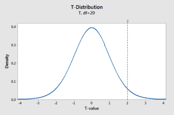
The tricky thing about $\mathrm{t}$-values is that they are difficult to interpret on their own. Imagine we performed a t-test, and it produced a t-value of 2. What does this t-value mean exactly?
We know that the sample mean doesn’t equal the null hypothesis value because this t-value doesn’t equal zero. We can also state that the effect is twice the variability. However, we don’t know how exceptional our value is if the null hypothesis is correct.
To be able to interpret individual t-values, we must place them in a larger context. T-distributions provide this broader context so we can determine the unusualness of an individual t-value.
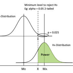
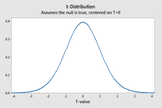
A single t-test produces a single t-value. Now, imagine the following process. First, let’s assume that the null hypothesis is true for the population. Now, suppose we repeat our study many times by drawing numerous random samples of the same size from this population. Next, we perform t-tests on all the samples and plot the distribution of the t-values. This distribution is known as a sampling distribution, which is a type of probability distribution.
If we follow this procedure, we produce a graph that displays the distribution of t-values that we obtain from a population where the null hypothesis is true. We use sampling distributions to calculate probabilities for how unusual our sample statistic is if the null hypothesis is true.
Luckily, we don’t need to go through the hassle of collecting numerous random samples to create this graph! Statisticians understand the properties of t-distributions so we can estimate the sampling distribution using the t-distribution and our sample size.
The degrees of freedom (DF) for the statistical design define the tdistribution for a particular study. We’ll go over degrees of freedom in more detail in a later chapter. For now, understand that degrees of freedom are closely related to the sample size. For t-tests, there is a different t-distribution for each sample size.
统计代写| 假设检验作业代写HYPOTHESIS TESTING代考|t-Distributions and Sample Size
The sample size for a t-test determines the degrees of freedom (DF) for that test, which specifies the t-distribution. The overall effect is that as the sample size decreases, the tails of the t-distribution become thicker. Thicker tails indicate that t-values are more likely to be far from zero even when the null hypothesis is correct. The changing shapes are how t-distributions factor in the greater uncertainty when you have a smaller sample.
You can see this effect in the probability distribution plot below that displays t-distributions for 5 and 30 DF.
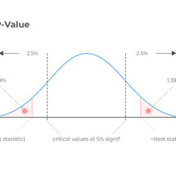
Sample means from smaller samples tend to be less precise. In other words, with a smaller sample, it’s less surprising to have an extreme tvalue, which affects the probabilities and p-values. A t-value of 2 has a p-value of $10.2 \%$ and $5.4 \%$ for 5 and $30 \mathrm{DF}$, respectively. Use larger samples!
统计代写| 假设检验作业代写HYPOTHESIS TESTING代考|Z-tests versus t-tests
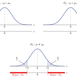
Z-tests are very similar to t-tests. You use both kinds of tests fo same reasons-comparing means. Both types of tests have one-sample, two-sample, and paired versions. They even have the same assumptions-with one major exception. That difference determines when you’ll use a Z-test versus t-test.
- Z-test: Use when you know the population standard deviation.
- t-Test: Use when you have an estimate of the population standard deviation.
I’m not covering Z-tests in this book for one excellent reason. You’ll never use one in practice!
Think about it. The Z-test assumes that you know the population standard deviation. That rarely happens. In what situation would you not know the population mean (hence, the need to test it), but yet you do know the population standard deviation? As I discussed earlier, these parameters are generally unknowable.
Despite this critical limitation, many statistics students learn about Ztests. Why is that? Many statistics textbooks use Z-tests because it is easier for students to calculate manually. However, the t-test is more accurate, particularly for smaller sample sizes. For more information about manually calculating Z-scores and using them to calculate probabilities, read my Introduction to Statistics ebook.
Z-tests use the standard normal distribution (mean $=0$, standard deviation $=1$ ) to calculate p-values while t-tests use the t-distribution. However, the t-distribution can approximate the normal distribution.
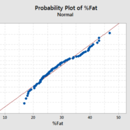
When statisticians say that a particular distribution approximates the normal distribution, it simply means that they have very similar shapes under certain conditions. T-distributions with at least 30 degrees of freedom will closely follow the normal distribution, as shown in the probability plot below. Using either of these distributions to calculate p-values will produce similar results.
假设检验代写
统计代写|假设检验作业代写HYPOTHESIS TESTING代考|T-DISTRIBUTIONS AND STATISTICAL SIGNIFICANCE
术语“t 检验”是指这些假设检验使用 t 值来评估您的样本数据这一事实。T 值是影响效应大小、样本大小和变异性的检验统计量。假设检验使用根据您的样本计算的检验统计量来将您的样本与原假设进行比较。如果检验统计量足够极端,这表明您的数据与原假设不相容,您可以拒绝原假设。
别担心。我发现这些统计术语的技术定义更容易用图表来解释,我们会明白的!
关于棘手的事情吨-values 是它们难以单独解释。想象一下,我们进行了 t 检验,它产生的 t 值为 2。这个 t 值究竟是什么意思?
我们知道样本均值不等于原假设值,因为这个 t 值不等于零。我们还可以说效果是可变性的两倍。但是,如果原假设是正确的,我们不知道我们的值有多特殊。
为了能够解释单个 t 值,我们必须将它们放在更大的上下文中。T 分布提供了更广泛的背景,因此我们可以确定单个 t 值的异常性。
单个 t 检验产生单个 t 值。现在,想象以下过程。首先,让我们假设原假设对总体是正确的。现在,假设我们通过从该人群中抽取大量相同大小的随机样本来重复我们的研究多次。接下来,我们对所有样本进行 t 检验并绘制 t 值的分布。这种分布称为抽样分布,是一种概率分布。
如果我们遵循这个过程,我们会生成一个图表,显示我们从零假设为真的总体中获得的 t 值的分布。我们使用抽样分布来计算如果原假设为真,我们的样本统计量有多不寻常的概率。
幸运的是,我们不需要费力地收集大量随机样本来创建这个图表!统计学家了解 t 分布的性质,因此我们可以使用 t 分布和我们的样本量来估计抽样分布。
自由度DF对于统计设计,定义特定研究的 t 分布。我们将在后面的章节中更详细地讨论自由度。现在,请了解自由度与样本量密切相关。对于 t 检验,每个样本量都有不同的 t 分布。
统计代写| 假设检验作业代写HYPOTHESIS TESTING代考|T-DISTRIBUTIONS AND SAMPLE SIZE
t 检验的样本量决定了自由度DF对于该测试,它指定了 t 分布。总体效果是随着样本量的减小,t 分布的尾部变得更粗。较粗的尾巴表明即使原假设正确,t 值也更有可能远离零。当样本较小时,变化的形状是 t 分布如何影响较大的不确定性。
您可以在下面显示 5 和 30 DF 的 t 分布的概率分布图中看到这种效果。
来自较小样本的样本均值往往不太精确。换句话说,对于较小的样本,有一个极值 t 值并不令人惊讶,它会影响概率和 p 值。t 值为 2 的 p 值为10.2%和5.4%对于 5 和30DF, 分别。使用更大的样本!
统计代写| 假设检验作业代写HYPOTHESIS TESTING代考|Z-TESTS VERSUS T-TESTS
Z 检验与 t 检验非常相似。您出于相同的原因使用这两种测试 – 比较方法。两种类型的测试都有单样本、双样本和配对版本。他们甚至有相同的假设——除了一个主要的例外。这种差异决定了您何时使用 Z 检验与 t 检验。
- Z 检验:当您知道总体标准差时使用。
- t 检验:当您估计总体标准差时使用。
出于一个很好的原因,我没有在本书中介绍 Z 检验。你永远不会在实践中使用一个!
想想看。Z 检验假设您知道总体标准差。这种情况很少发生。在什么情况下你会不知道人口的意思H和nC和,吨H和n和和d吨○吨和s吨一世吨,但你知道总体标准差吗?正如我之前所讨论的,这些参数通常是不可知的。
尽管有这个严重的限制,许多统计专业的学生还是学习了 Ztests。这是为什么?许多统计教科书使用 Z 检验,因为学生更容易手动计算。但是,t 检验更准确,特别是对于较小的样本量。有关手动计算 Z 分数和使用它们来计算概率的更多信息,请阅读我的统计简介电子书。
Z 检验使用标准正态分布米和一种n$=0$,s吨一种nd一种rdd和v一世一种吨一世○n$=1$在 t 检验使用 t 分布时计算 p 值。但是,t 分布可以逼近正态分布。
当统计学家说某个特定分布近似于正态分布时,它仅仅意味着它们在某些条件下具有非常相似的形状。具有至少 30 个自由度的 T 分布将紧密遵循正态分布,如下面的概率图所示。使用这些分布中的任何一个来计算 p 值都会产生类似的结果。

统计代写| 假设检验作业代写Hypothesis testing代考|Population Parameters vs. Sample Statistics 请认准UprivateTA™. UprivateTA™为您的留学生涯保驾护航。
统计代考
统计是汉语中的“统计”原有合计或汇总计算的意思。 英语中的“统计”(Statistics)一词来源于拉丁语status,是指各种现象的状态或状况。
数论代考
数论(number theory ),是纯粹数学的分支之一,主要研究整数的性质。 整数可以是方程式的解(丢番图方程)。 有些解析函数(像黎曼ζ函数)中包括了一些整数、质数的性质,透过这些函数也可以了解一些数论的问题。 透过数论也可以建立实数和有理数之间的关系,并且用有理数来逼近实数(丢番图逼近)
数值分析代考
数值分析(Numerical Analysis),又名“计算方法”,是研究分析用计算机求解数学计算问题的数值计算方法及其理论的学科。 它以数字计算机求解数学问题的理论和方法为研究对象,为计算数学的主体部分。
随机过程代写
随机过程,是依赖于参数的一组随机变量的全体,参数通常是时间。 随机变量是随机现象的数量表现,其取值随着偶然因素的影响而改变。 例如,某商店在从时间t0到时间tK这段时间内接待顾客的人数,就是依赖于时间t的一组随机变量,即随机过程
Matlab代写
MATLAB 是一种用于技术计算的高性能语言。它将计算、可视化和编程集成在一个易于使用的环境中,其中问题和解决方案以熟悉的数学符号表示。典型用途包括:数学和计算算法开发建模、仿真和原型制作数据分析、探索和可视化科学和工程图形应用程序开发,包括图形用户界面构建MATLAB 是一个交互式系统,其基本数据元素是一个不需要维度的数组。这使您可以解决许多技术计算问题,尤其是那些具有矩阵和向量公式的问题,而只需用 C 或 Fortran 等标量非交互式语言编写程序所需的时间的一小部分。MATLAB 名称代表矩阵实验室。MATLAB 最初的编写目的是提供对由 LINPACK 和 EISPACK 项目开发的矩阵软件的轻松访问,这两个项目共同代表了矩阵计算软件的最新技术。MATLAB 经过多年的发展,得到了许多用户的投入。在大学环境中,它是数学、工程和科学入门和高级课程的标准教学工具。在工业领域,MATLAB 是高效研究、开发和分析的首选工具。MATLAB 具有一系列称为工具箱的特定于应用程序的解决方案。对于大多数 MATLAB 用户来说非常重要,工具箱允许您学习和应用专业技术。工具箱是 MATLAB 函数(M 文件)的综合集合,可扩展 MATLAB 环境以解决特定类别的问题。可用工具箱的领域包括信号处理、控制系统、神经网络、模糊逻辑、小波、仿真等。