如果你也在 怎样代写概率论probability theory这个学科遇到相关的难题,请随时右上角联系我们的24/7代写客服。概率论probability theory作为统计学的数学基础,概率论对许多涉及数据定量分析的人类活动至关重要。概率论的方法也适用于对复杂系统的描述,只对其状态有部分了解,如在统计力学或顺序估计。二十世纪物理学的一个伟大发现是量子力学中描述的原子尺度的物理现象的概率性质。
概率论probability theory是与概率有关的数学分支。虽然有几种不同的概率解释,但概率论以严格的数学方式处理这一概念,通过一组公理来表达它。通常,这些公理以概率空间的形式表达概率,将一个取值在0和1之间的度量,称为概率度量,分配给一组称为样本空间的结果。样本空间的任何指定子集被称为事件。概率论的核心课题包括离散和连续随机变量、概率分布和随机过程(为非决定性或不确定的过程或测量量提供数学抽象,这些过程或测量量可能是单一发生的,或以随机方式随时间演变)。尽管不可能完美地预测随机事件,但对它们的行为可以有很多说法。概率论中描述这种行为的两个主要结果是大数法则和中心极限定理。
my-assignmentexpert™ 概率论probability theory作业代写,免费提交作业要求, 满意后付款,成绩80\%以下全额退款,安全省心无顾虑。专业硕 博写手团队,所有订单可靠准时,保证 100% 原创。my-assignmentexpert™, 最高质量的概率论probability theory作业代写,服务覆盖北美、欧洲、澳洲等 国家。 在代写价格方面,考虑到同学们的经济条件,在保障代写质量的前提下,我们为客户提供最合理的价格。 由于统计Statistics作业种类很多,同时其中的大部分作业在字数上都没有具体要求,因此概率论probability theory作业代写的价格不固定。通常在经济学专家查看完作业要求之后会给出报价。作业难度和截止日期对价格也有很大的影响。
想知道您作业确定的价格吗? 免费下单以相关学科的专家能了解具体的要求之后在1-3个小时就提出价格。专家的 报价比上列的价格能便宜好几倍。
my-assignmentexpert™ 为您的留学生涯保驾护航 在数学Mathematics作业代写方面已经树立了自己的口碑, 保证靠谱, 高质且原创的数学Mathematics代写服务。我们的专家在概率论probability theory代写方面经验极为丰富,各种概率论probability theory相关的作业也就用不着 说。
我们提供的概率论probability theory及其相关学科的代写,服务范围广, 其中包括但不限于:
数学代写|概率论代写probability theory代考|Previous estimation of dispersion
To obtain scale equivariant M-estimators of location, an intuitive approach is to use
$$
\widehat{\mu}=\arg \min {\mu} \sum{i=1}^{n} \rho\left(\frac{x_{i}-\mu}{\hat{\sigma}}\right),
$$
where $\hat{\sigma}$ is a previously computed dispersion estimator. It is easy to verify that $\hat{\mu}$ is indeed scale equivariant. Since $\hat{\sigma}$ does not depend on $\mu,(2.66)$ implies that $\hat{\mu}$ is a solution of
$$
\sum_{i=1}^{n} \psi\left(\frac{x_{i}-\hat{\mu}}{\hat{\sigma}}\right)=0
$$
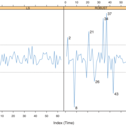
It is intuitive that $\hat{\sigma}$ must itself be robust. In Example 1.2, using (2.66) with bisquare $\psi$ with $k=4.68$, and $\hat{\sigma}=\operatorname{MADN}(\mathbf{x})$, yields $\hat{\mu}=25.56$; using $\hat{\sigma}=\operatorname{SD}(\mathbf{x})$ instead gives $\hat{\mu}=25.12$. Now add to the dataset three copies of the lowest value, $-44$. The results change to $26.42$ and $17.19$. The reason for this change is that the outliers “inflate” the SD, and hence the location estimator attributes to them too much weight.
Note that since $k$ is chosen in order to ensure a given efficiency for the unit normal, if we want $\hat{\mu}$ to attain the same efficiency for any normal, $\hat{\sigma}$ must “estimate the SD at the normal”, in the sense that if the data are $\mathrm{N}\left(\mu, \sigma^{2}\right)$, then when $n \rightarrow \infty, \hat{\sigma}$ tends in probability to $\sigma$. This is why we use the normalized median absolute deviation MADN described previously, rather than the un-normalized version MAD.
If a number $m>n / 2$ of data values are concentrated at a single value $x_{0}$, we have $\operatorname{MAD}(\mathbf{x})=0$, and hence the estimator is not defined. In this case we define $\widehat{\mu}=x_{0}=\operatorname{Med}(\mathbf{x})$. Besides being intuitively plausible, this definition can be justified by a limit argument. Let the $n$ data values be different, and let $m$ of them tend to $x_{0}$. Then it is not difficult to show that, in the limit, the solution of $(2.66)$ is $x_{0}$.
It can be proved that if $F$ is symmetric, then when $n$ is large, $\hat{\mu}$ behaves as if $\hat{\sigma}$ were constant, in the following sense: if $\hat{\sigma}$ tends in probability to $\sigma$, then the distribution of $\hat{\mu}$ is approximately normal with variance (2.65) (for asymmetric $F$ the asymptotic variance is more complicated; see Section 10.6). Therefore the efficiency of $\hat{\mu}$ does not depend on that of $\hat{\sigma}$. In Chapter 3 it will be seen, however, that its robustness does depend on that of $\hat{\sigma}$.
数学代写|概率论代写probability theory代考|Simultaneous M-estimators of location and dispersion
An alternative approach is to consider a location-dispersion model with two unknown parameters
$$
x_{i}=\mu+\sigma u_{i}
$$
where $u_{i}$ has density $f_{0}$, and hence $x_{i}$ has density
$$
f(x)=\frac{1}{\sigma} f_{0}\left(\frac{x-\mu}{\sigma}\right) .
$$In this case, $\sigma$ is the scale parameter of the random variables $\sigma u_{i}$, but it is a dispersion parameter for the $x_{i}$.
We now derive the simultaneous MLE of $\mu$ and $\sigma$ in model (2.69):
$$
(\widehat{\mu}, \hat{\sigma})=\arg \max {\mu, \sigma} \frac{1}{\sigma^{n}} \prod{i=1}^{n} f_{0}\left(\frac{x_{i}-\mu}{\sigma}\right)
$$
which can be written as
$$
(\hat{\mu}, \hat{\sigma})=\arg \min {\mu, \sigma}\left{\frac{1}{n} \sum{i=1}^{n} \rho_{0}\left(\frac{x_{i}-\mu}{\sigma}\right)+\log \sigma\right}
$$
with $\rho_{0}=-\log f_{0}$. The main point of interest here is $\mu$, while $\sigma$ is a “nuisance parameter”.
概率论代写
数学代写|概率论代写PROBABILITY THEORY代考|PREVIOUS ESTIMATION OF DISPERSION
为了获得位置的尺度等变 M 估计量,一种直观的方法是使用
$$
\widehat{\mu}=\arg \min {\mu} \sum{i=1}^{n} \rho\left(\frac{x_{i}-\mu}{\hat{\sigma}}\right),
$$
where $\hat{\sigma}$ is a previously computed dispersion estimator. It is easy to verify that $\hat{\mu}$ is indeed scale equivariant. Since $\hat{\sigma}$ does not depend on $\mu,(2.66)$ implies that $\hat{\mu}$ is a solution of
$$
\sum_{i=1}^{n} \psi\left(\frac{x_{i}-\hat{\mu}}{\hat{\sigma}}\right)=0
$$
直观的是σ^本身必须是健壮的。在示例 1.2 中,使用2.66双正方形ψ和ķ=4.68, 和σ^=疯狂(X), 产量μ^=25.56; 使用σ^=标清(X)而是给出μ^=25.12. 现在将最小值的三个副本添加到数据集,−44. 结果变为26.42和17.19. 这种变化的原因是异常值“膨胀”了 SD,因此位置估计器对它们的权重过大。
请注意,由于ķ选择是为了确保单位正常的给定效率,如果我们想要μ^在任何正常情况下达到相同的效率,σ^必须“在正常情况下估计 SD”,即如果数据是ñ(μ,σ2),那么当n→∞,σ^倾向于σ. 这就是为什么我们使用前面描述的归一化中值绝对偏差 MADN,而不是未归一化版本的 MAD。
如果一个数米>n/2的数据值集中在一个值上X0, 我们有疯狂的(X)=0,因此没有定义估计量。在这种情况下,我们定义μ^=X0=和(X). 除了直观合理之外,这个定义还可以通过极限论证来证明。让n数据值不同,让米其中倾向于X0. 那么不难证明,在极限下,(2.66)是X0.
可以证明,如果F是对称的,那么当n很大,μ^表现得好像σ^在以下意义上是恒定的:如果σ^倾向于σ, 那么分布μ^近似正态,有方差2.65 F这r一种s是米米和吨r一世C$F$吨H和一种s是米p吨这吨一世C在一种r一世一种nC和一世s米这r和C这米pl一世C一种吨和d;s和和小号和C吨一世这n10.6. 因此效率μ^不依赖于σ^. 然而,在第 3 章中将会看到,它的稳健性确实取决于σ^.
数学代写|概率论代写PROBABILITY THEORY代考|SIMULTANEOUS M-ESTIMATORS OF LOCATION AND DISPERSION
另一种方法是考虑具有两个未知参数的位置分散模型
X一世=μ+σ在一世
在哪里在一世有密度F0, 因此X一世有密度
F(X)=1σF0(X−μσ).在这种情况下,σ是随机变量的尺度参数σ在一世, 但它是一个色散参数X一世.
我们现在推导出同时 MLEμ和σ在模型中2.69:
$$
(\widehat{\mu}, \hat{\sigma})=\arg \max {\mu, \sigma} \frac{1}{\sigma^{n}} \prod{i=1}^{n} f_{0}\left(\frac{x_{i}-\mu}{\sigma}\right)
$$
which can be written as
$$
(\hat{\mu}, \hat{\sigma})=\arg \min {\mu, \sigma}\left{\frac{1}{n} \sum{i=1}^{n} \rho_{0}\left(\frac{x_{i}-\mu}{\sigma}\right)+\log \sigma\right}
$$
与ρ0=−日志F0. 这里的主要兴趣点是μ, 尽管σ是一个“讨厌的参数”。

数学代写|概率论代写probability theory代考 请认准UprivateTA™. UprivateTA™为您的留学生涯保驾护航。
电磁学代考
物理代考服务:
物理Physics考试代考、留学生物理online exam代考、电磁学代考、热力学代考、相对论代考、电动力学代考、电磁学代考、分析力学代考、澳洲物理代考、北美物理考试代考、美国留学生物理final exam代考、加拿大物理midterm代考、澳洲物理online exam代考、英国物理online quiz代考等。
光学代考
光学(Optics),是物理学的分支,主要是研究光的现象、性质与应用,包括光与物质之间的相互作用、光学仪器的制作。光学通常研究红外线、紫外线及可见光的物理行为。因为光是电磁波,其它形式的电磁辐射,例如X射线、微波、电磁辐射及无线电波等等也具有类似光的特性。
大多数常见的光学现象都可以用经典电动力学理论来说明。但是,通常这全套理论很难实际应用,必需先假定简单模型。几何光学的模型最为容易使用。
相对论代考
上至高压线,下至发电机,只要用到电的地方就有相对论效应存在!相对论是关于时空和引力的理论,主要由爱因斯坦创立,相对论的提出给物理学带来了革命性的变化,被誉为现代物理性最伟大的基础理论。
流体力学代考
流体力学是力学的一个分支。 主要研究在各种力的作用下流体本身的状态,以及流体和固体壁面、流体和流体之间、流体与其他运动形态之间的相互作用的力学分支。
随机过程代写
随机过程,是依赖于参数的一组随机变量的全体,参数通常是时间。 随机变量是随机现象的数量表现,其取值随着偶然因素的影响而改变。 例如,某商店在从时间t0到时间tK这段时间内接待顾客的人数,就是依赖于时间t的一组随机变量,即随机过程
Matlab代写
MATLAB 是一种用于技术计算的高性能语言。它将计算、可视化和编程集成在一个易于使用的环境中,其中问题和解决方案以熟悉的数学符号表示。典型用途包括:数学和计算算法开发建模、仿真和原型制作数据分析、探索和可视化科学和工程图形应用程序开发,包括图形用户界面构建MATLAB 是一个交互式系统,其基本数据元素是一个不需要维度的数组。这使您可以解决许多技术计算问题,尤其是那些具有矩阵和向量公式的问题,而只需用 C 或 Fortran 等标量非交互式语言编写程序所需的时间的一小部分。MATLAB 名称代表矩阵实验室。MATLAB 最初的编写目的是提供对由 LINPACK 和 EISPACK 项目开发的矩阵软件的轻松访问,这两个项目共同代表了矩阵计算软件的最新技术。MATLAB 经过多年的发展,得到了许多用户的投入。在大学环境中,它是数学、工程和科学入门和高级课程的标准教学工具。在工业领域,MATLAB 是高效研究、开发和分析的首选工具。MATLAB 具有一系列称为工具箱的特定于应用程序的解决方案。对于大多数 MATLAB 用户来说非常重要,工具箱允许您学习和应用专业技术。工具箱是 MATLAB 函数(M 文件)的综合集合,可扩展 MATLAB 环境以解决特定类别的问题。可用工具箱的领域包括信号处理、控制系统、神经网络、模糊逻辑、小波、仿真等。