物理代考| Classical Optics 量子力学代写

物理代考| Classical Optics 量子力学代写

物理代写

1.1 Classical Optics
Consider a non-dispersive wave which is the real part of
$$
\Psi(x, t)=e^{i(k x-\omega t)}=e^{i k(x-c t)} \quad ; \omega=k c
$$
Here $c$ is the velocity of the wave, and the frequency and wavelength are related by
$$
\omega=2 \pi \nu=k c=2 \pi \frac{c}{\lambda}
$$
As we have seen, this could be an electromagnetic wave in vacuum, a transverse wave on a string under tension, or the sound wave in a medium. This wave satisfies the wave equation
$$
\frac{\partial^{2} \Psi(x, t)}{\partial x^{2}}=\frac{1}{c^{2}} \frac{\partial^{2} \Psi(x, t)}{\partial t^{2}} \quad ; \text { wave equation }
$$
We have also seen that a linear combination of two such waves with slightly different wavenumbers $k$, produces an amplitude modulated signal. A more general linear combination can produce a localized wave packet, or pulse.

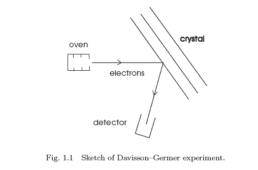
Huygen’s principle states that each point on a wavefront acts as a source of an outgoing spherical wave. From this, and its generalizations, one derives single-slit diffraction, two-slit and multi-slit interference, and most of classical wave optics. ${ }^{1}$
${ }^{1}$ See Probs. 1.1-1.2. For a more detailed discussion here, see [Wiki (2021)].
1
2
Introduction to Quantum Mechanics
1.2 Planck Distribution
Early in the twentieth century, Planck was studying the distribution of energy as a function of frequency for the electromagnetic radiation in a cavity. Normal modes are uncoupled simple harmonic oscillators. The classical equipartition theorem says that the energy of a simple harmonic oscillator at an absolute temperature $T$ is
where $k_{B}$ is Boltzmann’s constant $$ k_{B}=1.381 \times 10^{-23} \mathrm{~J} /{ }^{\circ} \mathrm{K} \quad ; \text { Boltzmann’s constant } $$ the frequency, this classical result says there should be an ever-increasing energy as a function of frequency for the radiation in a cavity, the so-called ultraviolet catastrophe. ${ }^{2}$

To fit his data, Planck employed an empirical expression of the form
$$
\langle\varepsilon(\nu)\rangle=\frac{h \nu}{e^{h \nu / k_{B} T}-1} \quad ; \text { Planck distribution }
$$
where $h$ is a constant obtained from the fit, now known as Planck’s constant
$$
\frac{h}{2 \pi} \equiv \hbar=1.055 \times 10^{-34} \mathrm{Js} \quad ; \text { Planck’s constant }
$$
Note that at low frequency, the Planck distribution reproduces the equipartition result
$$
\frac{h \nu}{e^{h \nu / k_{B} T}-1} \rightarrow k_{B} T \quad ; h \nu \ll k_{B} T
$$
while at high frequency, it now disappears exponentially
$$
\frac{h \nu}{e^{h \nu / k_{B} T}-1} \rightarrow h \nu e^{-h \nu / k_{B} T} \quad ; h \nu \gg k_{B} T
$$
$$
\frac{h \nu}{e^{h \nu / k_{B} T}-1} \rightarrow h \nu e^{-h \nu / k_{B} T} \quad ; h \nu \gg k_{B} T
$$
One can ask where this empirical Planck distribution might come from. Suppose that in each mode with frequency $\nu$ in the cavity it is possible to have any number $n$ of photons, each with energy
‘ See Prob. 1.3.
3 Then the mean energy in the mode at the temperature an elementary statistical calculation with the Boltzmann $e^{-n h \nu / k_{B} T}$ as $$ \begin{array}{l}\text { Motivation } \ \qquad \varepsilon(\nu)\rangle=\frac{\sum_{n=0}^{\infty}(n h \nu) e^{-n h \nu / k_{B} T}}{\sum_{n=0}^{\infty} e^{-n h \nu / k_{B} T}} \ \qquad=-\frac{d}{d\left(1 / k_{B} T\right)} \ln \left(\sum_{n=0}^{\infty} e^{-n h \nu / k_{B} T}\right) \ \text { The photons of light each have an energy } \ \text { The sum is just a geometric series }^{3} \ \qquad \sum_{n=0}^{\infty} x^{n}=\frac{1}{1.3}\end{array} $$

We know the momentum flux in an electromagnetic wave is $1 / c$ times the energy flux, and hence each photon in light also has a momentum
$$
p=\frac{h \nu}{c} \quad ; \text { photon }
$$
Photons are now observed every day in the laboratory as single events in low-intensity radiation detectors.
${ }^{3}$ Note $e^{-n h \nu / k_{B} T}=\left(e^{-h \nu / k_{B} T}\right)^{n} .$

物理代考

1.1 经典光学
考虑一个非色散波，它是
$$
\Psi(x, t)=e^{i(k x-\omega t)}=e^{i k(x-c t)} \quad ; \omega=k c
$$
这里$c$是波的速度，频率和波长的关系为
$$
\omega=2 \pi \nu=k c=2 \pi \frac{c}{\lambda}
$$
正如我们所见，这可能是真空中的电磁波、受拉弦上的横波或介质中的声波。该波满足波动方程
$$
\frac{\partial^{2} \Psi(x, t)}{\partial x^{2}}=\frac{1}{c^{2}} \frac{\partial^{2} \Psi (x, t)}{\partial t^{2}} \quad ; \text { 波动方程 }
$$
我们还看到，具有略微不同波数 $k$ 的两个此类波的线性组合会产生幅度调制信号。更一般的线性组合可以产生局部波包或脉冲。

惠更斯原理指出，波前的每个点都充当出射球面波的源。由此及其推广，可以推导出单缝衍射、双缝和多缝干涉以及大多数经典波动光学。 ${ }^{1}$
${ }^{1}$ 见问题。 1.1-1.2。有关此处更详细的讨论，请参阅 [Wiki (2021)]。
1
2
量子力学导论
1.2 普朗克分布
20 世纪初，普朗克正在研究腔内电磁辐射的能量分布与频率的函数关系。正常模式是非耦合的简单谐振子。经典均分定理说，简单谐振子在绝对温度 $T$ 下的能量为
其中 $k_{B}$ 是玻尔兹曼常数 $$ k_{B}=1.381 \times 10^{-23} \mathrm{~J} /{ }^{\circ} \mathrm{K} \quad ; \text { 玻尔兹曼常数 } $$ 频率，这个经典结果表明腔内的辐射应该有一个不断增加的能量作为频率的函数，即所谓的紫外线灾难。 ${ }^{2}$

为了拟合他的数据，普朗克采用了以下形式的经验表达式
$$
\langle\varepsilon(\nu)\rangle=\frac{h \nu}{e^{h \nu / k_{B} T}-1} \quad ; \text { 普朗克分布 }
$$
其中 $h$ 是从拟合中获得的常数，现在称为普朗克常数
$$
\frac{h}{2 \pi} \equiv \hbar=1.055 \times 10^{-34} \mathrm{Js} \quad ; \text { 普朗克常数 }
$$
请注意，在低频下，普朗克分布再现了均分结果
$$
\frac{h \nu}{e^{h \nu / k_{B} T}-1} \rightarrow k_{B} T \quad ; h \nu \ll k_{B} T
$$
在高频下，它现在呈指数级消失
$$
\frac{h \nu}{e^{h \nu / k_{B} T}-1} \rightarrow h \nu e^{-h \nu / k_{B} T} \quad ; h \nu \gg k_{B} T
$$
$$
\frac{h \nu}{e^{h \nu / k_{B} T}-1} \rightarrow h \nu e^{-h \nu / k_{B} T} \quad ; h \nu \gg k_{B} T
$$
人们可以问这种经验普朗克分布可能来自哪里。假设在腔中频率为 $\nu$ 的每个模式中，可能有任意数量的 $n$ 个光子，每个光子都有能量
‘见概率。 1.3.
3 然后在温度下模态的平均能量用玻尔兹曼 $e^{-nh \nu / k_{B} T}$ 作为 $$ \begin{array}{l}\text { Motivation } \ \qquad \varepsilon(\nu)\rangle=\frac{\sum_{n=0}^{\infty}(nh \nu) e^{-nh \nu / k_{B} T}}{\ sum_{n=0}^{\infty} e^{-nh \nu / k_{B} T}} \ \qquad=-\frac{d}{d\left(1 / k_{B} T\ right)} \ln \left(\sum_{n=0}^{\infty} e^{-nh \nu / k_{B} T}\right) \ \text { 每个光子都有一个能量} \ \text { 总和只是一个几何级数 }^{3} \ \qquad \sum_{n=0}^{\infty} x^{n}=\frac{1}{1.3}\end {数组} $$

我们知道电磁波中的动量通量是能量通量的 1/c$ 倍，因此光中的每个光子也具有动量
$$
p=\frac{h \nu}{c} \quad ; \文本{光子}
$$
现在每天在实验室中都在低强度辐射探测器中观察到光子作为单个事件。
${ }^{3}$ 注意 $e^{-nh \nu / k_{B} T}=\left(e^{-h \nu / k_{B} T}\right)^{n} 。 $

物理代考| Classical Optics量子力学代写 请认准UprivateTA™. UprivateTA™为您的留学生涯保驾护航。

电磁学代考

物理代考服务：
物理Physics考试代考、留学生物理online exam代考、电磁学代考、热力学代考、相对论代考、电动力学代考、电磁学代考、分析力学代考、澳洲物理代考、北美物理考试代考、美国留学生物理final exam代考、加拿大物理midterm代考、澳洲物理online exam代考、英国物理online quiz代考等。

光学代考

光学（Optics），是物理学的分支，主要是研究光的现象、性质与应用，包括光与物质之间的相互作用、光学仪器的制作。光学通常研究红外线、紫外线及可见光的物理行为。因为光是电磁波，其它形式的电磁辐射，例如X射线、微波、电磁辐射及无线电波等等也具有类似光的特性。

大多数常见的光学现象都可以用经典电动力学理论来说明。但是，通常这全套理论很难实际应用，必需先假定简单模型。几何光学的模型最为容易使用。

相对论代考

上至高压线，下至发电机，只要用到电的地方就有相对论效应存在！相对论是关于时空和引力的理论，主要由爱因斯坦创立，相对论的提出给物理学带来了革命性的变化，被誉为现代物理性最伟大的基础理论。

流体力学代考

流体力学是力学的一个分支。 主要研究在各种力的作用下流体本身的状态，以及流体和固体壁面、流体和流体之间、流体与其他运动形态之间的相互作用的力学分支。

随机过程代写

随机过程，是依赖于参数的一组随机变量的全体，参数通常是时间。 随机变量是随机现象的数量表现，其取值随着偶然因素的影响而改变。 例如，某商店在从时间t0到时间tK这段时间内接待顾客的人数，就是依赖于时间t的一组随机变量，即随机过程

Matlab代写