如果你也在 怎样代写金融计量经济学Financial Econometrics ECON335这个学科遇到相关的难题,请随时右上角联系我们的24/7代写客服。金融计量经济学Financial Econometrics是使用统计方法来发展理论或检验经济学或金融学的现有假设。计量经济学依靠的是回归模型和无效假设检验等技术。计量经济学也可用于尝试预测未来的经济或金融趋势。
金融计量经济学Financial Econometrics的一个基本工具是多元线性回归模型。计量经济学理论使用统计理论和数理统计来评估和发展计量经济学方法。计量经济学家试图找到具有理想统计特性的估计器,包括无偏性、效率和一致性。应用计量经济学使用理论计量经济学和现实世界的数据来评估经济理论,开发计量经济学模型,分析经济历史和预测。
金融计量经济学Financial Econometrics 免费提交作业要求, 满意后付款,成绩80\%以下全额退款,安全省心无顾虑。专业硕 博写手团队,所有订单可靠准时,保证 100% 原创。 最高质量的金融计量经济学Financial Econometrics作业代写,服务覆盖北美、欧洲、澳洲等 国家。 在代写价格方面,考虑到同学们的经济条件,在保障代写质量的前提下,我们为客户提供最合理的价格。 由于作业种类很多,同时其中的大部分作业在字数上都没有具体要求,因此金融计量经济学Financial Econometrics作业代写的价格不固定。通常在专家查看完作业要求之后会给出报价。作业难度和截止日期对价格也有很大的影响。
同学们在留学期间,都对各式各样的作业考试很是头疼,如果你无从下手,不如考虑my-assignmentexpert™!
my-assignmentexpert™提供最专业的一站式服务:Essay代写,Dissertation代写,Assignment代写,Paper代写,Proposal代写,Proposal代写,Literature Review代写,Online Course,Exam代考等等。my-assignmentexpert™专注为留学生提供Essay代写服务,拥有各个专业的博硕教师团队帮您代写,免费修改及辅导,保证成果完成的效率和质量。同时有多家检测平台帐号,包括Turnitin高级账户,检测论文不会留痕,写好后检测修改,放心可靠,经得起任何考验!
想知道您作业确定的价格吗? 免费下单以相关学科的专家能了解具体的要求之后在1-3个小时就提出价格。专家的 报价比上列的价格能便宜好几倍。
我们在经济Economy代写方面已经树立了自己的口碑, 保证靠谱, 高质且原创的经济Economy代写服务。我们的专家在微观经济学Microeconomics代写方面经验极为丰富,各种微观经济学Microeconomics相关的作业也就用不着 说。
经济代写|计量经济学代写Econometrics代考|Limitations of the Best Linear Projection
Let’s compare the linear projection and linear CEF models.
From Theorem 2.4.4 we know that the CEF error has the property $\mathbb{E}[X e]=0$. Thus a linear $\mathrm{CEF}$ is the best linear projection. However, the converse is not true as the projection error does not necessarily satisfy $\mathbb{E}[e \mid X]=0$. Furthermore, the linear projection may be a poor approximation to the CEF.
To see these points in a simple example, suppose that the true process is $Y=X+X^{2}$ with $X \sim \mathrm{N}(0,1)$. In this case the true CEF is $m(x)=x+x^{2}$ and there is no error. Now consider the linear projection of $Y$ on $X$ and a constant, namely the model $Y=\beta X+\alpha+e$. Since $X \sim \mathrm{N}(0,1)$ then $X$ and $X^{2}$ are uncorrelated and the linear projection takes the form $\mathscr{P}[Y \mid X]=X+1$. This is quite different from the true $\mathrm{CEF} m(X)=$ $X+X^{2}$. The projection error equals $e=X^{2}-1$ which is a deterministic function of $X$ yet is uncorrelated with $X$. We see in this example that a projection error need not be a CEF error and a linear projection can be a poor approximation to the CEF.
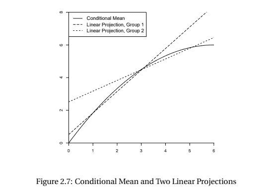
Another defect of linear projection is that it is sensitive to the marginal distribution of the regressors when the conditional mean is nonlinear. We illustrate the issue in Figure $2.7$ for a constructed ${ }^{11}$ joint distribution of $Y$ and $X$. The solid line is the nonlinear CEF of $Y$ given $X$. The data are divided in two groups – Group 1 and Group 2-which have different marginal distributions for the regressor $X$, and Group 1 has a lower mean value of $X$ than Group 2. The separate linear projections of $Y$ on $X$ for these two groups are displayed in the figure by the dashed lines. These two projections are distinct approximations to the CEF. A defect with linear projection is that it leads to the incorrect conclusion that the effect of $X$ on $Y$ is different for individuals in the two groups. This conclusion is incorrect because in fact there is no difference in the conditional mean function. The apparent difference is a by-product of linear approximations to a nonlinear mean combined with different marginal distributions for the conditioning variables.
经济代写|计量经济学代写Econometrics代考|Random Coefficient Model
A model which is notationally similar to but conceptually distinct from the linear CEF model is the linear random coefficient model. It takes the form $Y=X^{\prime} \eta$ where the individual-specific coefficient $\eta$ is random and independent of $X$. For example, if $X$ is years of schooling and $Y$ is log wages, then $\eta$ is the individual-specific returns to schooling. If a person obtains an extra year of schooling, $\eta$ is the actual change in their wage. The random coefficient model allows the returns to schooling to vary in the population. Some individuals might have a high return to education (a high $\eta$ ) and others a low return, possibly 0 , or even negative.
In the linear CEF model the regressor coefficient equals the regression derivative – the change in the conditional mean due to a change in the regressors, $\beta=\nabla m(X)$. This is not the effect on a given individual, it is the effect on the population average. In contrast, in the random coefficient model the random vector $\eta=\nabla\left(X^{\prime} \eta\right)$ is the true causal effect – the change in the response variable $Y$ itself due to a change in the regressors.
It is interesting, however, to discover that the linear random coefficient model implies a linear CEF. To see this, let $\beta=\mathbb{E}[\eta]$ and $\Sigma=\operatorname{var}[\eta]$ denote the mean and covariance matrix of $\eta$ and then decompose the random coefficient as $\eta=\beta+u$ where $u$ is distributed independently of $X$ with mean zero and covariance matrix $\Sigma$. Then we can write
$$
\mathbb{E}[Y \mid X]=X^{\prime} \mathbb{E}[\eta \mid X]=X^{\prime} \mathbb{E}[\eta]=X^{\prime} \beta
$$
so the CEF is linear in $X$, and the coefficient $\beta$ equals the mean of the random coefficient $\eta$.
We can thus write the equation as a linear $\operatorname{CEF} Y=X^{\prime} \beta+e$ where $e=X^{\prime} u$ and $u=\eta-\beta$. The error is conditionally mean zero: $\mathbb{E}[e \mid X]=0$. Furthermore
$$
\operatorname{var}[e \mid X]=X^{\prime} \operatorname{var}[\eta] X=X^{\prime} \Sigma X
$$
so the error is conditionally heteroskedastic with its variance a quadratic function of $X$.
计量经济学代写
经济代写|计量经济学代写ECONOMETRICS代考|LIMITATIONS OF THE BEST LINEAR PROJECTION
让我们比较一下线性投影和线性 CEF 模型。
由定理 2.4.4 我们知道 $C E F$ 误差具有性质 $\mathbb{E}[X e]=0$. 因此一个线性CEF是最好的线性投影。然而,反之则不成立,因为投影误差不一定满足 $\mathbb{E}[e \mid X]=0$. 此外,
线性投影可能不是 $\mathrm{CEF}$ 的近似值。
为了在一个简单的例子中看到这些点,假设真正的过程是 $Y=X+X^{2}$ 和 $X \sim \mathrm{N}(0,1)$. 在这种情况下,真正的 $\mathrm{CEF}$ 是 $m(x)=x+x^{2}$ 并且没有错误。现在考慮线
性投影 $Y$ 上 $X$ 和一个常数,即模型 $Y=\beta X+\alpha+e$. 自从 $X \sim \mathrm{N}(0,1)$ 然后 $X$ 和 $X^{2}$ 是不相关的,线性投影的形式为 $\mathscr{P}[Y \mid X]=X+1$. 这与真真实情况大相径庭
$\mathrm{CEF} m(X)=X+X^{2}$. 投影洖差等于 $e=X^{2}-1$ 这是一个确定性函数 $X$ 然而与 $X$. 我们在这个例子中看到,投影误差不一定是 $\mathrm{CEF}$ 误差,线性投影可能不是 $\mathrm{CEF}$
的近似值。
线性投影的另一个缺陷是当条件均值非线性时,它对回归量的边际分布很敏感。我们在图中说明了这个问题 $2.7$ 对于一个构造 11 联合分布 $Y$ 和 $X$. 实线是非线性 CEF
$Y$ 给定 $X$. $\frac{1}{2}$ 据分为两组-第 1 组和第 2 组 – 回归量具有不同的边际分布 $X$ ,并且第 1 组的平均值较低 $X$ 比组 2 . 的单独线性投影 $Y$ 上 $X$ 这两组在图中用虚线表示。这
两个预测是 CEF 的不同近似值。线性投影的一个缺陷是它会导致错误的结论,即 $X$ 上 $Y$ 两组中的个体不同。这个结论是不正确的,因为实际上条件均值函数没有区
别。明显的差异是非线性均值的线性近似与条件变量的不同边际分布相结合的副产品。
经济代写|计量经济学代写ECONOMETRICS代考|RANDOM COEFFICIENT MODEL
一个在符昊上与线性 CEF 模型相似但在概念上不同的模型是线性随机系数模型。它采用以下形式 $Y=X^{\prime} \eta$ 其中个体特定系数 $\eta$ 是随机的并且独立于 $X$. 例如,如果 $X$ 是受教育年限和 $Y$ 是对数工资,那么 $\eta$ 是个人特定的教育回报。如果一个人获得额外一年的学业, $\eta$ 是他们工资的实际变化。随机系数模型允许受教育的回报因人口 而异。有些人可能有很高的教育回报ahigh\$\$\$和其他低回报,可能是 0 ,甚至是负数。
在线性 CEF 模型中,回归杀数等于回归导数 – 由于回归变量的变化导致条件均值的变化, $\beta=\nabla m(X)$. 这不是对特定个体的影响,而是对总体平均数的影响。相 反,在随机系数模型中,随机向量 $\eta=\nabla\left(X^{\prime} \eta\right)$ 是真正的因果效应一一响应变量的变化 $Y$ 本身是由于回归变量的变化。
然而,有趣的是发现线性随机系数模型意味着线性 CEF。要看到这一点,让 $\beta=\mathbb{E}[\eta]$ 和 $\Sigma=\operatorname{var}[\eta]$ 表示均值和协方差矩阵 $\eta$ 然后将随机系数分解为 $\eta=\beta+u$ 在哪 里 $u$ 是独立分布的 $X$ 均值为零和协方差矩阵 $\Sigma$. 然后我们可以写
$$
\mathbb{E}[Y \mid X]=X^{\prime} \mathbb{E}[\eta \mid X]=X^{\prime} \mathbb{E}[\eta]=X^{\prime} \beta
$$
所以 CEF 是线性的 $X$, 和系数 $\beta$ 等于随机系数的平均值 $\eta$.
因此,我们可以将方程写成线性 $\mathrm{CEF} Y=X^{\prime} \beta+e$ 在哪里 $e=X^{\prime} u$ 和 $u=\eta-\beta$. 误差在条件下为零: $\mathbb{E}[e \mid X]=0$. 此外
$$
\operatorname{var}[e \mid X]=X^{\prime} \operatorname{var}[\eta] X=X^{\prime} \Sigma X
$$
所以误差是条件异方差的,它的方差是一个二次函数 $X$.

经济代写|计量经济学代考ECONOMETRICS代考 请认准UprivateTA™. UprivateTA™为您的留学生涯保驾护航。
微观经济学代写
微观经济学是主流经济学的一个分支,研究个人和企业在做出有关稀缺资源分配的决策时的行为以及这些个人和企业之间的相互作用。my-assignmentexpert™ 为您的留学生涯保驾护航 在数学Mathematics作业代写方面已经树立了自己的口碑, 保证靠谱, 高质且原创的数学Mathematics代写服务。我们的专家在图论代写Graph Theory代写方面经验极为丰富,各种图论代写Graph Theory相关的作业也就用不着 说。
线性代数代写
线性代数是数学的一个分支,涉及线性方程,如:线性图,如:以及它们在向量空间和通过矩阵的表示。线性代数是几乎所有数学领域的核心。
博弈论代写
现代博弈论始于约翰-冯-诺伊曼(John von Neumann)提出的两人零和博弈中的混合策略均衡的观点及其证明。冯-诺依曼的原始证明使用了关于连续映射到紧凑凸集的布劳威尔定点定理,这成为博弈论和数学经济学的标准方法。在他的论文之后,1944年,他与奥斯卡-莫根斯特恩(Oskar Morgenstern)共同撰写了《游戏和经济行为理论》一书,该书考虑了几个参与者的合作游戏。这本书的第二版提供了预期效用的公理理论,使数理统计学家和经济学家能够处理不确定性下的决策。
微积分代写
微积分,最初被称为无穷小微积分或 “无穷小的微积分”,是对连续变化的数学研究,就像几何学是对形状的研究,而代数是对算术运算的概括研究一样。
它有两个主要分支,微分和积分;微分涉及瞬时变化率和曲线的斜率,而积分涉及数量的累积,以及曲线下或曲线之间的面积。这两个分支通过微积分的基本定理相互联系,它们利用了无限序列和无限级数收敛到一个明确定义的极限的基本概念 。
计量经济学代写
什么是计量经济学?
计量经济学是统计学和数学模型的定量应用,使用数据来发展理论或测试经济学中的现有假设,并根据历史数据预测未来趋势。它对现实世界的数据进行统计试验,然后将结果与被测试的理论进行比较和对比。
根据你是对测试现有理论感兴趣,还是对利用现有数据在这些观察的基础上提出新的假设感兴趣,计量经济学可以细分为两大类:理论和应用。那些经常从事这种实践的人通常被称为计量经济学家。
Matlab代写
MATLAB 是一种用于技术计算的高性能语言。它将计算、可视化和编程集成在一个易于使用的环境中,其中问题和解决方案以熟悉的数学符号表示。典型用途包括:数学和计算算法开发建模、仿真和原型制作数据分析、探索和可视化科学和工程图形应用程序开发,包括图形用户界面构建MATLAB 是一个交互式系统,其基本数据元素是一个不需要维度的数组。这使您可以解决许多技术计算问题,尤其是那些具有矩阵和向量公式的问题,而只需用 C 或 Fortran 等标量非交互式语言编写程序所需的时间的一小部分。MATLAB 名称代表矩阵实验室。MATLAB 最初的编写目的是提供对由 LINPACK 和 EISPACK 项目开发的矩阵软件的轻松访问,这两个项目共同代表了矩阵计算软件的最新技术。MATLAB 经过多年的发展,得到了许多用户的投入。在大学环境中,它是数学、工程和科学入门和高级课程的标准教学工具。在工业领域,MATLAB 是高效研究、开发和分析的首选工具。MATLAB 具有一系列称为工具箱的特定于应用程序的解决方案。对于大多数 MATLAB 用户来说非常重要,工具箱允许您学习和应用专业技术。工具箱是 MATLAB 函数(M 文件)的综合集合,可扩展 MATLAB 环境以解决特定类别的问题。可用工具箱的领域包括信号处理、控制系统、神经网络、模糊逻辑、小波、仿真等。