如果你也在 怎样代写金融统计Financial Statistics MS&E349这个学科遇到相关的难题,请随时右上角联系我们的24/7代写客服。金融统计Financial Statistics数据包括所有总结过去行为或预测单个金融证券、一组证券或广泛地理区域内市场未来行为的数字数据。首先将这些统计数据归入三个领域之一是很有用的。在宏观层面上,它有助于了解一个国家的财政状况和衡量经济增长。 阅读更多。在微观层面上,统计帮助分析师确定一个公司的商业收入,收益。就个人而言,它包括工资或薪金或其他付款。
金融统计Financial Statistics第二大类金融统计数据评估的是证券市场的行为。大多数金融市场发达的国家都有各种指数,追踪整体市场活动或特定市场部分的活动。在美国,这些指数的例子有道琼斯工业平均指数、标准/普尔500指数和纽约证券交易所综合指数。其他例子包括英国的金融时报100指数,日本的日经225指数和法国的CAC40指数。这些被广泛关注的指数中的每一个都在追踪一般的市场状况。市场指数可以通过其构建方法或其包含的证券样本来区分。
金融统计Financial Statistics代写,免费提交作业要求, 满意后付款,成绩80\%以下全额退款,安全省心无顾虑。专业硕 博写手团队,所有订单可靠准时,保证 100% 原创。最高质量的金融统计Financial Statistics作业代写,服务覆盖北美、欧洲、澳洲等 国家。 在代写价格方面,考虑到同学们的经济条件,在保障代写质量的前提下,我们为客户提供最合理的价格。 由于作业种类很多,同时其中的大部分作业在字数上都没有具体要求,因此金融统计Financial Statistics作业代写的价格不固定。通常在专家查看完作业要求之后会给出报价。作业难度和截止日期对价格也有很大的影响。
同学们在留学期间,都对各式各样的作业考试很是头疼,如果你无从下手,不如考虑my-assignmentexpert™!
my-assignmentexpert™提供最专业的一站式服务:Essay代写,Dissertation代写,Assignment代写,Paper代写,Proposal代写,Proposal代写,Literature Review代写,Online Course,Exam代考等等。my-assignmentexpert™专注为留学生提供Essay代写服务,拥有各个专业的博硕教师团队帮您代写,免费修改及辅导,保证成果完成的效率和质量。同时有多家检测平台帐号,包括Turnitin高级账户,检测论文不会留痕,写好后检测修改,放心可靠,经得起任何考验!
想知道您作业确定的价格吗? 免费下单以相关学科的专家能了解具体的要求之后在1-3个小时就提出价格。专家的 报价比上列的价格能便宜好几倍。
我们在统计Statistics代写方面已经树立了自己的口碑, 保证靠谱, 高质且原创的统计Statistics代写服务。我们的专家在金融统计Financial Statistics代写方面经验极为丰富,各种金融统计Financial Statistics相关的作业也就用不着说。
数据科学代写|金融统计代写Financial Statistics代考|Engle (2002) Dynamic Conditional Correlation Model
Let $r_{t}=\left(r_{1 t}, \ldots, r_{n t}\right)$ represent a $(n \times 1)$ vector of financial assets returns at time $(\mathrm{t})$. Moreover, let $\varepsilon_{t}$ $=\left(\varepsilon_{1 t}, \ldots, \varepsilon_{n t}\right)$ be a $(n \times 1)$ vector of error terms obtained from an estimated system of mean equations for these return series.
Engle (2002) proposes the following decomposition for the conditional variance-covariance matrix of asset returns:
$$
H_{t}=D_{t} R_{t} D_{t}
$$
where $D_{t}$ is a $(n \times n)$ diagonal matrix of time-varying standard deviations from univariate Garch models, and $R_{t}$ is a $(n \times n)$ time-varying correlation matrix of asset returns $\left(\rho_{i j,} t\right)$.
The conditional variance-covariance matrix $\left(H_{t}\right)$ displayed in equation [1] is estimated in two steps. In the first step, univariate Garch $(1,1)$ models are applied to mean returns equations, thus obtaining conditional variance estimates for each financial asset $\left(\sigma^{2}\right.$ it; for $\left.i=1,2, \ldots ., n\right)$, namely:
$$
\sigma_{i t}^{2}=\sigma^{2} U_{i t}\left(1-\lambda_{1 i}-\lambda_{2 i}\right)+\lambda_{1 i} \sigma_{i, t-1}^{2}+\lambda_{2 i} \varepsilon_{i, t-1}^{2}
$$
where $\sigma^{2}$ uit is the unconditional variance of the ith asset return, $\lambda_{1 i}$ is the volatility persistence parameter, and $\lambda_{2 i}$ is the parameter capturing the influence of past errors on the conditional variance.
In the second step, the residuals vector obtained from the mean equations system $\left(\varepsilon_{t}\right)$ is divided by the corresponding estimated standard deviations, thus obtaining standardized residuals (i.e., $u_{i t}=$ $\varepsilon_{i t} / \sqrt{\sigma_{i, t}^{2}}$ for $\mathrm{i}=1,2, \ldots ., n$ ), which are subsequently used to estimate the parameters governing the time-varying correlation matrix.
More specifically, the dynamic conditional correlation matrix of asset returns may be expressed as:
$$
Q_{t}=\left(1-\delta_{1}-\delta_{2}\right) \bar{Q}+\delta_{1} Q_{t-1}+\delta_{2}\left(u_{t-1} u_{t-1}^{\prime}\right)
$$
where $\overline{\mathrm{Q}}=\mathrm{E}\left[u_{t} u_{t}^{\prime}\right]$ is the $(n \times n)$ unconditional covariance matrix of standardized residuals, and $\delta_{1}$ and $\delta_{2}$ are parameters (capturing, respectively, the persistence in correlation dynamics and the impact of past shocks on current conditional correlations). ${ }^{2}$
数据科学代写|金融统计代写Financial Statistics代考|Model Estimation and Dynamic Conditional Correlation Patterns
The econometric framework summarized by Equations (1)-(3) was applied to gold, oil, and exchange rate returns.
After a preliminary data inspection, and in line with many contributions relying on this approach (see e.g., Ding and Vo (2012) and Jain and Biswal (2016) with regards to “safe haven” assets), a VAR(1) specification was selected to model the mean returns equation system. Alternative filtering procedures (such as an $\mathrm{AR}(1)$ specification for return series) produced substantially identical results.
The VAR(1) specification was selected on the basis of the Akaike Information Criterion (AIC) and of Likelihood Ratio tests against higher-order VAR models. Diagnostic tests on residuals from the VAR(1) specification never rejected the null of absence of serial correlation, while rejecting the normality assumption. This rejection was consistent with the preliminary data analysis, where the Jarque and Bera (1980) statistics turned out to be strongly significant.
These departures from normality have relevant implications on the distributional assumptions underlying the Multivariate Garch DCC model. More specifically, instead of relying on the standard Gaussian assumption (as in Engle (2002) seminal model), it is advisable to assume a Multivariate $\mathrm{t}$-distribution in order to better capture the fat-tailed nature of asset returns. This is the approach taken in the present paper. ${ }^{3}$
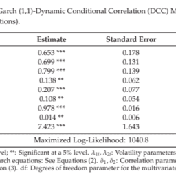
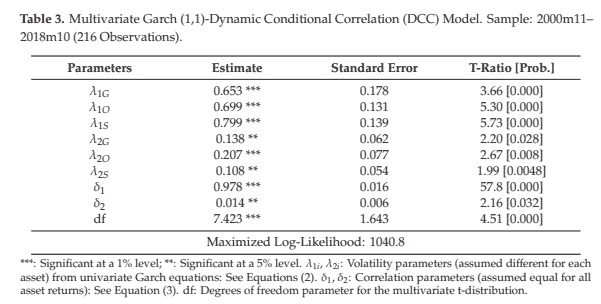
With regards to parameters, conditional volatility coefficients were unrestricted, and assumed different for each asset (see Equation (2)). Conditional correlation coefficients were unrestricted as well, although a common correlation structure was imposed in model’s estimation (see Equation (3))).
The Maximum Likelihood estimator converged after 48 iterations and relied on 216 observations (20 observations were used to initialize the recursions).
Table 3 contains the results.
金融统计代写
数据科学代写|金融统计代写FINANCIAL STATISTICS代 考|ENGLE (2002) DYNAMIC CONDITIONAL CORRELATION MODEL
让 $r_{t}=\left(r_{1 t}, \ldots, r_{n t}\right)$ 代表一个 $(n \times 1)$ 金融资产回报向量 $(\mathrm{t})$. 此外,让 $\varepsilon_{t}=\left(\varepsilon_{1 t}, \ldots, \varepsilon_{n t}\right)$ 做一个 $(n \times 1)$ 从这些回报序列的估计平均方程系统获得的误差项向量。 恩格尔 2002 对资产收益的条件方差-协方差矩阵提出以下分解:
$$
H_{t}=D_{t} R_{t} D_{t}
$$
在哪里 $D_{t}$ 是一个 $(n \times n)$ 来自单变量 $G a r c h$ 模型的时变标准差的对角矩阵,以及 $R_{t}$ 是一个 $(n \times n)$ 资产收益的时变相关矩阵 $\left(\rho_{i j}, t\right)$.
条件方差-协方差矩阵 $\left(H_{t}\right)$ 显示在方程式中
估计分两步。第一步,单变量 $\operatorname{Garch}(1,1)$ 模型应用于平均收益方程,从而获得每个金融资产的条件方差估计 $\left(\sigma^{2}\right.$ 它; 为了 $\left.i=1,2, \ldots, n\right)$ ,即:
$$
\sigma_{i t}^{2}=\sigma^{2} U_{i t}\left(1-\lambda_{1 i}-\lambda_{2 i}\right)+\lambda_{1 i} \sigma_{i, t-1}^{2}+\lambda_{2 i} \varepsilon_{i, t-1}^{2}
$$
在哪里 $\sigma^{2}$ uit 是第 $\mathrm{i}$ 个资产收益的无条件方差, $\lambda_{1 i}$ 是波动率持久性参数,并且 $\lambda_{2 i}$ 是捕捉过去误差对条件方差的影响的参数。
第二步,从均值方程组得到的残差向量 $\left(\varepsilon_{t}\right)$ 除以相应的估计标准差,从而获得标准化残差 $i . e ., \$ u_{i t}=\$ \$ \varepsilon_{i t} / \sqrt{\sigma_{i, t}^{2}} \$ f o r \$ \mathrm{i}=1,2, \ldots, n \$$, 随后用于估计控制时变 相关矩阵的参数。
更具体地说,资产收益的动态条件相关矩阵可以表示为:
$$
Q_{t}=\left(1-\delta_{1}-\delta_{2}\right) \bar{Q}+\delta_{1} Q_{t-1}+\delta_{2}\left(u_{t-1} u_{t-1}^{\prime}\right)
$$
在哪里 $\overline{\mathrm{Q}}=\mathrm{E}\left[u_{t} u_{t}^{\prime}\right]$ 是个 $(n \times n)$ 标准化残差的无条件协方差矩阵,以及 $\delta_{1}$ 和 $\delta_{2}$ 是参数
capturing, respectively, thepersistenceincorrelationdynamicsandtheimpactofpastshocksoncurrentconditionalcorrelations ${ }^{2}$. $^{2}$.
数据科学代写|金融统计代写FINANCIAL STATISTICS代 考|MODEL ESTIMATION AND DYNAMIC CONDITIONAL CORRELATION PATTERNS
Equations 总结的计量经济学框妿1-3适用于昔金、石油和汇率回报。 程系统。萺代过滤程序suchasanSAR(1\$返回系列的规格) 产生了基本相同的结果。
VAR1规格是根据 Akaike 信息标准选择的 $A I C$ 以及针对高阶 VAR 模型的似然比检验。VAR残差的诊断测试1规范从不拒绝不存在序列相关的零点,同时拒绝正态性假 设。这一拒绝与初步数据分析一致,其中 Jarque 和 Bera1980统计结果证明是非常重要的。
这些偏离正态性对多元 Garch DCC 模型的分布假设具有相关影响。更具体地说,而不是依赖于标准的高斯假设 $a s i n E n g l e(2002$ 开创性模型),建议假设一个多变 量t-分配以更好地捕捉资产回报的肥尾性质。这是本文所采用的方法。
在参数方面,条件波动系数不受限制,并假设每种资产不同seeEquation(2)。条件相关系数也不受限制,尽管在模型的估计中采用了共同的相关结构
seeEquation(3) )。
最大似然估计量在 48 次迭代后收敛并依赖于 216 次观察 20 observationswereusedtoinitializetherecursions.
表 3 包含结果。

数据科学代写|金融统计代写Financial Statistics代考 请认准UprivateTA™. UprivateTA™为您的留学生涯保驾护航。
微观经济学代写
微观经济学是主流经济学的一个分支,研究个人和企业在做出有关稀缺资源分配的决策时的行为以及这些个人和企业之间的相互作用。my-assignmentexpert™ 为您的留学生涯保驾护航 在数学Mathematics作业代写方面已经树立了自己的口碑, 保证靠谱, 高质且原创的数学Mathematics代写服务。我们的专家在图论代写Graph Theory代写方面经验极为丰富,各种图论代写Graph Theory相关的作业也就用不着 说。
线性代数代写
线性代数是数学的一个分支,涉及线性方程,如:线性图,如:以及它们在向量空间和通过矩阵的表示。线性代数是几乎所有数学领域的核心。
博弈论代写
现代博弈论始于约翰-冯-诺伊曼(John von Neumann)提出的两人零和博弈中的混合策略均衡的观点及其证明。冯-诺依曼的原始证明使用了关于连续映射到紧凑凸集的布劳威尔定点定理,这成为博弈论和数学经济学的标准方法。在他的论文之后,1944年,他与奥斯卡-莫根斯特恩(Oskar Morgenstern)共同撰写了《游戏和经济行为理论》一书,该书考虑了几个参与者的合作游戏。这本书的第二版提供了预期效用的公理理论,使数理统计学家和经济学家能够处理不确定性下的决策。
微积分代写
微积分,最初被称为无穷小微积分或 “无穷小的微积分”,是对连续变化的数学研究,就像几何学是对形状的研究,而代数是对算术运算的概括研究一样。
它有两个主要分支,微分和积分;微分涉及瞬时变化率和曲线的斜率,而积分涉及数量的累积,以及曲线下或曲线之间的面积。这两个分支通过微积分的基本定理相互联系,它们利用了无限序列和无限级数收敛到一个明确定义的极限的基本概念 。
计量经济学代写
什么是计量经济学?
计量经济学是统计学和数学模型的定量应用,使用数据来发展理论或测试经济学中的现有假设,并根据历史数据预测未来趋势。它对现实世界的数据进行统计试验,然后将结果与被测试的理论进行比较和对比。
根据你是对测试现有理论感兴趣,还是对利用现有数据在这些观察的基础上提出新的假设感兴趣,计量经济学可以细分为两大类:理论和应用。那些经常从事这种实践的人通常被称为计量经济学家。
Matlab代写
MATLAB 是一种用于技术计算的高性能语言。它将计算、可视化和编程集成在一个易于使用的环境中,其中问题和解决方案以熟悉的数学符号表示。典型用途包括:数学和计算算法开发建模、仿真和原型制作数据分析、探索和可视化科学和工程图形应用程序开发,包括图形用户界面构建MATLAB 是一个交互式系统,其基本数据元素是一个不需要维度的数组。这使您可以解决许多技术计算问题,尤其是那些具有矩阵和向量公式的问题,而只需用 C 或 Fortran 等标量非交互式语言编写程序所需的时间的一小部分。MATLAB 名称代表矩阵实验室。MATLAB 最初的编写目的是提供对由 LINPACK 和 EISPACK 项目开发的矩阵软件的轻松访问,这两个项目共同代表了矩阵计算软件的最新技术。MATLAB 经过多年的发展,得到了许多用户的投入。在大学环境中,它是数学、工程和科学入门和高级课程的标准教学工具。在工业领域,MATLAB 是高效研究、开发和分析的首选工具。MATLAB 具有一系列称为工具箱的特定于应用程序的解决方案。对于大多数 MATLAB 用户来说非常重要,工具箱允许您学习和应用专业技术。工具箱是 MATLAB 函数(M 文件)的综合集合,可扩展 MATLAB 环境以解决特定类别的问题。可用工具箱的领域包括信号处理、控制系统、神经网络、模糊逻辑、小波、仿真等。