如果你也在 怎样代写金融衍生品Financial Derivatives BA4825/5825这个学科遇到相关的难题,请随时右上角联系我们的24/7代写客服。金融衍生品Financial Derivatives是金融工具的三大类之一,另外两类是股权(即股票或股份)和债权(即债券和抵押贷款)。历史上最古老的衍生品例子,由亚里士多德证明,被认为是古希腊哲学家泰勒斯签订的橄榄合同交易,他在交换中获利。1936年被取缔的桶装水商店是一个较近的历史例子。
金融衍生品Financial Derivatives在金融领域,衍生品是一种合同,其价值来自于一个基础实体的表现。衍生品可用于多种目的,包括对价格变动进行保险(套期保值),为投机增加价格变动的风险,或进入其他难以交易的资产或市场。一些更常见的衍生品包括远期、期货、期权、掉期,以及这些的变体,如合成抵押债务和信用违约掉期。大多数衍生品在场外(场外)或芝加哥商品交易所等交易所进行交易,而大多数保险合同已经发展成为一个独立的行业。在美国,在2007-2009年的金融危机之后,将衍生品转移到交易所进行交易的压力越来越大。
金融衍生品Financial Derivatives代写,免费提交作业要求, 满意后付款,成绩80\%以下全额退款,安全省心无顾虑。专业硕 博写手团队,所有订单可靠准时,保证 100% 原创。最高质量的金融衍生品Financial Derivatives作业代写,服务覆盖北美、欧洲、澳洲等 国家。 在代写价格方面,考虑到同学们的经济条件,在保障代写质量的前提下,我们为客户提供最合理的价格。 由于作业种类很多,同时其中的大部分作业在字数上都没有具体要求,因此金融衍生品Financial Derivatives作业代写的价格不固定。通常在专家查看完作业要求之后会给出报价。作业难度和截止日期对价格也有很大的影响。
同学们在留学期间,都对各式各样的作业考试很是头疼,如果你无从下手,不如考虑my-assignmentexpert™!
my-assignmentexpert™提供最专业的一站式服务:Essay代写,Dissertation代写,Assignment代写,Paper代写,Proposal代写,Proposal代写,Literature Review代写,Online Course,Exam代考等等。my-assignmentexpert™专注为留学生提供Essay代写服务,拥有各个专业的博硕教师团队帮您代写,免费修改及辅导,保证成果完成的效率和质量。同时有多家检测平台帐号,包括Turnitin高级账户,检测论文不会留痕,写好后检测修改,放心可靠,经得起任何考验!
想知道您作业确定的价格吗? 免费下单以相关学科的专家能了解具体的要求之后在1-3个小时就提出价格。专家的 报价比上列的价格能便宜好几倍。
金融代写|金融衍生品代写Financial Derivatives代考|HISTORICAL SIMULATION
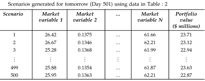
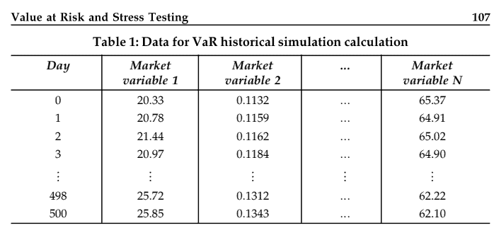
Historical simulation is one popular way of estimating VaR. It involves using past data in a very direct way as a guide to what might happen in the future. Suppose that we wish to calculate VaR for a portfolio using a one-day time horizon, a $99 \%$ confidence level, and 500 days of data. The first step is to identify the market variables affecting the portfolio. These will typically be exchange rates, equity prices, interest rates, and so on. We then collect data on the movements in these market variables over the most recent 500 days. This provides us with 500 alternative scenarios for what can happen between today and tomorrow. Scenario 1 is where the percentage changes in the values of all variables are the same as they were on the first day for which we have collected data;scenario 2 is where they are the same as on the second day for which we have data; and so on. Foreach scenario we calculate the dollar change in the value of the portfolio between today andtomorrow. This defines a probability distribution for daily changes in the value of our portfolio.The fifth-worst daily change is the first percentile of the distribution. The estimate of $\mathrm{VaR}$ is theloss when we are at this first percentile point. Assuming that the last 500 days are a good guide towhat could happen during the next day, we are $99 \%$ certain that we will not take a loss greater thanour VaR estimate.The historical simulation methodology is illustrated in Tables 1 and .2. Table .1 showsobservations on market variables over the last 500 days. The observations are taken at someparticular point in time during the day (usually the close of trading). We denote the first day forwhich we have data as Day 0; the second as Day 1; and so on. Today is Day 500; tomorrow isDay 501. Table 2 shows the values of the. market variables tomorrow if their percentage changesbetween today and tomorrow are the same as they were between Day $\mathrm{i}-1$ and Day i for $1<\mathrm{i}^{\prime} \wedge 500$. The first row in Table 16.2 shows the values of market variables tomorrow assuming their percentage changes between today and tomorrow are the same as they were between Day 0 and Day 1 ; the second row shows the values of market variables tomorrow assuming theirpercentage changes between Day 1 and Day 2 occur; and so on. The 500 rows in Table 2 arethe 500 scenarios considered.Define $\mathrm{i}$; as the value of a market variable on Day $\mathrm{i}$ and suppose that today is Day $\mathrm{m}$. The ithscenario assumes that the value of the market variable tomorrow will be
$$
v_m \frac{v_i}{v_i-1}
$$
In our example, $m=500$. For the first variable, the value today, v500, is 25.85 . Also $\mathrm{v} 0=20.33$ and $\mathrm{V} \backslash=20.78$. It follows that the value of the first market variable in the first scenario is
$$
25,5 \times \$^{\wedge}=26.42
$$
金融代写|金融衍生品代写Financial Derivatives代考|MODEL-BUILDING APPROACH
The main alternative to historical simulation is the model-building approach (sometimes alsocalled the variance-covariance approach). Before getting into the details of the approach, it isappropriate to mention one issue concerned with the units for measuring volatility.
Daily Volatilities
In option pricing we usually measure time in years, and the volatility of an asset is usually quotedas a “volatility per year”. When using the model-building approach to calculate VaR, we usuallymeasure time in days and the volatility of an asset is usually quoted as a “volatility per day”. What is the relationship between the volatility per year used in option pricing and the volatilityper day used in VaR calculations? Let us define oyr as the volatility per year of a certain asset and TOday as the equivalent volatility per day of the asset. Assuming 252 trading days in a year, we canuse equation to write the standard deviation of the continuously compounded return on theasset in one year as either $\mathrm{a}{\mathrm{yr}}$ or $\mathrm{c}{1 \text { day }} \backslash / 252$. It follows that so that daily volatility is about $6 \%$ of annual volatility. As pointed out in Section 12.4, $\mathrm{a}{\mathrm{d} d \mathrm{dy}}$ is approximately equal to the standard deviation of the percentage change in the asset price in one day. For the purposes of calculating VaR, we assume exact equality. We define the daily volatility of an asset price (or any other variable) as equal to the standard deviation of the percentage change in one day. Our discussion in the next few sections assumes that we have estimates of daily volatilities and correlations. we explain how the estimates are produced. $$ \begin{aligned} \sigma{y r} & =\sigma_{y r \sigma_{d a y} \sqrt{252}} \
\sigma_{\text {day }} & =\frac{\sigma_{y r}}{V \overline{252}}
\end{aligned}
$$
金融衍生品代写
金融代写|金融衍生品代写FINANCIAL DERIVATIVES代考|HISTORICAL SIMULATION
历史模拟是估计 VaR 的一种流行方法。它涉及以非常直接的方式使用过去的数据作为末来可能发生的事情的指南。假设我们希望使用一天的时间 范围计算投资组合的 VaR,a99\%置信度和 500 天的数据。第一步是确定影响投资组合的市场变量。这些通常是汇率、股票价格、利率等。然后, 我们收集最近 500 天内这些市场变量变动的数据。这为我们提供了 500 种今天和明天之间可能发生的情况的替代方案。情景 1 是所有变量值的百分 比变化与我们收集数据的第一天相同;情景 2 是它们与我们有数据的第二天相同;等等。对于每种情况,我们计算今天和明天之间投资组合价值 的美元变化。这定义了我们投资组合价值每日变化的概率分布。第五差的每日变化是分布的第一个百分位数。的估计 $V a R$ 是我们处于第一个百分 位点时的损失。假设过去 500 天是第二天可能发生的事情的良好指南,我们是 $99 \%$ 确定我们不会承受大于我们的 VaR估计的损失。历史模拟方法 如表 1 和. 2 所示。表.1显示了过去 500 天对市场变量的观察。观察是在一天中的某个特定时间点进行的usuallythecloseoftrading. 我们将拥有 数据的第一天表示为第 0 天;第二个作为第 1 天;等等。今天是第 500 天;明天是第 501 天。表 2 显示了这些值。明天的市场变量,如果它们在今 天和明天之间的百分比变化与一天之间的变化相同 $\mathrm{i}-1$ 和第一天 $1<\mathrm{i}^{\prime} \wedge 500$. 表 16.2 中的第一行显示明天市场变量的值,假设它们在今天和明天 之间的百分比变化与第 0 天和第 1 天之间的百分比变化相同;第二行显示明天市场变量的值,假设它们在第 1 天和第 2 天之间发生百分比变化;等 等。表 2 中的 500 行是考虑的 500 个场景。定义i; 作为 Day 的市场变量值 1 假设今天是 Daym. 第 ith 个场景假设明天市场变量的值为
$$
v_m \frac{v_i}{v_i-1}
$$
在我们的例子中, $m=500$. 对于第一个变量,今天的值 $\mathrm{v} 500$ 是 25.85 。还 $\mathrm{v} 0=20.33$ 和 $\backslash=20.78$. 因此,第一种情况下第一个市场变量的值 为
$$
25,5 \times \$^{\wedge}=26.42
$$
金融代写|金融衍生品代写FINANCIAL DERIVATIVES代考|MODEL-BUILDING APPROACH
历史模拟的主要替代方法是模型构建方法sometimesalsocalledthevariance – covarianceapproach. 在深入探讨该方法的细节之前,有必要 提及一个与衡量波动率的单位有关的问题。
每日波动率
在期权定价中,我们通常以年为单位衡量时间,资产的波动率通常被引用为“每年的波动率”。在使用建模方法计算 VaR 时,我们通常以天为单位 来衡量时间,资产的波动率通常被引用为 “每天的波动率”。期权定价中使用的每年波动率与VaR计算中使用的每天波动率之间有什么关系? 让我 们将 oyr 定义为某种资产每年的波动率,将 TOday 定义为该资产每天的等效波动率。假设一年有 252 个交易日,我们可以用方程将资产在一年内的 连续复合收益的标准差写为 $a y r$ 或者 $\mathrm{c} 1$ day $\backslash / 252$. 由此可见,每日波动率约为 $6 \%$ 年度波动率。正如第 12.4 节所指出的, $\operatorname{ad} d \mathrm{dy}$ 约等于一天内资 产价格变化百分比的标准差。为了计算 VaR,我们假设完全相等。我们定义资产价格的每日波动率oranyothervariable等于一天内百分比变化的 标准差。我们在接下来几节中的讨论假设我们已经估计了每日波动率和相关性。我们解释了这些估计是如何产生的。
$$
\sigma y r=\sigma_{y r \sigma_{d a y} \sqrt{252}} \sigma_{\text {day }} \quad=\frac{\sigma_{y r}}{V \overline{252}}
$$

金融代写|金融衍生品代写Financial Derivatives代考 请认准UprivateTA™. UprivateTA™为您的留学生涯保驾护航。
微观经济学代写
微观经济学是主流经济学的一个分支,研究个人和企业在做出有关稀缺资源分配的决策时的行为以及这些个人和企业之间的相互作用。my-assignmentexpert™ 为您的留学生涯保驾护航 在数学Mathematics作业代写方面已经树立了自己的口碑, 保证靠谱, 高质且原创的数学Mathematics代写服务。我们的专家在图论代写Graph Theory代写方面经验极为丰富,各种图论代写Graph Theory相关的作业也就用不着 说。
线性代数代写
线性代数是数学的一个分支,涉及线性方程,如:线性图,如:以及它们在向量空间和通过矩阵的表示。线性代数是几乎所有数学领域的核心。
博弈论代写
现代博弈论始于约翰-冯-诺伊曼(John von Neumann)提出的两人零和博弈中的混合策略均衡的观点及其证明。冯-诺依曼的原始证明使用了关于连续映射到紧凑凸集的布劳威尔定点定理,这成为博弈论和数学经济学的标准方法。在他的论文之后,1944年,他与奥斯卡-莫根斯特恩(Oskar Morgenstern)共同撰写了《游戏和经济行为理论》一书,该书考虑了几个参与者的合作游戏。这本书的第二版提供了预期效用的公理理论,使数理统计学家和经济学家能够处理不确定性下的决策。
微积分代写
微积分,最初被称为无穷小微积分或 “无穷小的微积分”,是对连续变化的数学研究,就像几何学是对形状的研究,而代数是对算术运算的概括研究一样。
它有两个主要分支,微分和积分;微分涉及瞬时变化率和曲线的斜率,而积分涉及数量的累积,以及曲线下或曲线之间的面积。这两个分支通过微积分的基本定理相互联系,它们利用了无限序列和无限级数收敛到一个明确定义的极限的基本概念 。
计量经济学代写
什么是计量经济学?
计量经济学是统计学和数学模型的定量应用,使用数据来发展理论或测试经济学中的现有假设,并根据历史数据预测未来趋势。它对现实世界的数据进行统计试验,然后将结果与被测试的理论进行比较和对比。
根据你是对测试现有理论感兴趣,还是对利用现有数据在这些观察的基础上提出新的假设感兴趣,计量经济学可以细分为两大类:理论和应用。那些经常从事这种实践的人通常被称为计量经济学家。
Matlab代写
MATLAB 是一种用于技术计算的高性能语言。它将计算、可视化和编程集成在一个易于使用的环境中,其中问题和解决方案以熟悉的数学符号表示。典型用途包括:数学和计算算法开发建模、仿真和原型制作数据分析、探索和可视化科学和工程图形应用程序开发,包括图形用户界面构建MATLAB 是一个交互式系统,其基本数据元素是一个不需要维度的数组。这使您可以解决许多技术计算问题,尤其是那些具有矩阵和向量公式的问题,而只需用 C 或 Fortran 等标量非交互式语言编写程序所需的时间的一小部分。MATLAB 名称代表矩阵实验室。MATLAB 最初的编写目的是提供对由 LINPACK 和 EISPACK 项目开发的矩阵软件的轻松访问,这两个项目共同代表了矩阵计算软件的最新技术。MATLAB 经过多年的发展,得到了许多用户的投入。在大学环境中,它是数学、工程和科学入门和高级课程的标准教学工具。在工业领域,MATLAB 是高效研究、开发和分析的首选工具。MATLAB 具有一系列称为工具箱的特定于应用程序的解决方案。对于大多数 MATLAB 用户来说非常重要,工具箱允许您学习和应用专业技术。工具箱是 MATLAB 函数(M 文件)的综合集合,可扩展 MATLAB 环境以解决特定类别的问题。可用工具箱的领域包括信号处理、控制系统、神经网络、模糊逻辑、小波、仿真等。