统计代写|STAT501 Regression Analysis

A regression analysis relating test scores $(Y)$ to training hours $(X)$ produced the following fitted question: $\hat{y}=25-0.5 x$.
(a) What is the fitted value of the response variable corresponding to $x=7$ ?
Solution: The fitted value at $x=7$ is
$$
\hat{y}=25-(0.5)(7)=25-3.5=21.5 \text {. }
$$
(b) What is the residual corresponding to the data point with $x=3$ and $y=30$ ?
Solution: The fitted value corresponding to the data point with $x=3$ is
$$
\hat{y}=25-(0.5)(3)=25-1.5=23.5 .
$$
The residual corresponding to the data point with $x=3$ and $y=30$ is thus
$$
e_i=30-23.5=6.5 .
$$
(c) If $x$ increases 3 units, how does $\hat{y}$ change?
Solution: For increase of 1 in $x, \hat{y}$ changes by the slope. Therefore, if $x$ increase by 3 units, $\hat{y}$ will decrease by 3 times the slope, i.e. by $(3)(-0.5)=-1.5$.
(d) An additional test score is to obtained for a new observation at $x=6$. Would the test score for the new observation necessarily be 22? Explain.
Solution: Not necessarily. The new observation is a random variable from a normal distribution with estimated mean 22 . So you would not likely see the observation 22 .
(e) The error sums of squares $(S S E$ ) for this model was found to be 7 . If there were $n=16$ observations, provide the best estimate for $\sigma^2$.
Solution: The estimate of $\sigma^2$ is given by
$$
s^2=M S E=\frac{S S E}{d f_E}=\frac{S S E}{n-2}=\frac{7}{14}=0.5 .
$$
(f) Rewrite the regression equation in terms of $x^$ where $x^$ is training time measured in seconds. Show that your answer makes sense, i.e., gives the same predictions as the original equation (an example is sufficient).
Solution: If $x$ is the time in hours and $x^$ is the time in seconds, then $x^=60^2 x$. Therefore, $x=x^* / 3600$. The regression equation $\hat{Y}=25-0.5 x$ thus becomes $\hat{y}=25-0.5 \frac{x^}{3600}=25-0.0001389 x^$ (approximately).
For example, if $x=2$ hours, then $x^*=7200$ seconds. The original equation would give $\hat{y}=25-0.5(2)=24$, and the equation would give $\hat{y}=15-$ $0.0001389(24)=14.99667$. Thus, except for rounding error, the two equations give the same answer.

Explain the different between the following two equations:
$$
\begin{aligned}
& \hat{Y}=b_0+b_1 X \
& Y=\beta_0+\beta_1 X+\epsilon .
\end{aligned}
$$

Solution: The first equation is the fitted regression line which describes the linear relationship between the mean of the response variable (fitted value) and the explanatory variable $X$. The second equation is the linear model which describes the relationship between the observed $(X, Y)$ pairs. Not all the pairs will fall directly on a line as they will in the first equation, as indicated by the error term. In the first equation, the values $b_0$ and $b_1$ are known values obtained from the data, while in the second equation, the parameters $\beta_1$ and $\beta_0$ are unknown.

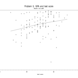
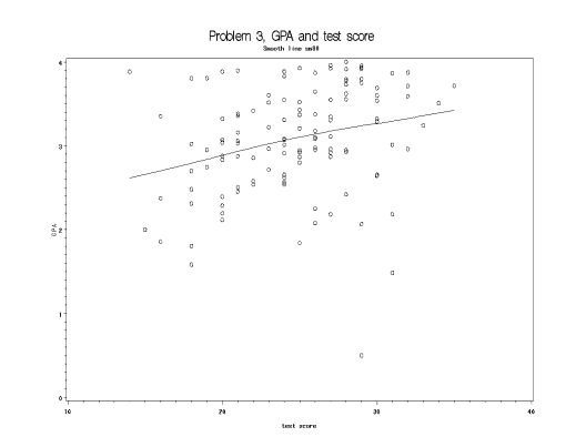
For this problem, use the “grade point average” data described in NKNW Problem #1.19. The data are on the disk that accompanies the text and can also be found on the class web site (CHO1PR19.DAT). Make sure you understand which column is $X$ and which is $Y$ and read in the data accordingly. See Topic 1 or nknw060. sas for an example of how to read in a data file.
(a) Plot the data using proc gplot. Include a smoothed function on the plot by preceding the plot statement with “SYMBOL1 $i=$ smNN” where NN is a number between 1 and 99. Note that larger numbers cause greater smoothing. Make sure to indicate the smoothing number in the title of the plot. Is the relationship approximately linear?
Solution: The relationship looks approximately linear. (See graph).
(b) Run a linear regression to predict GPA based on the entrance exam. Give the complete ANOVA table for this regression.
Solution: The included table shows that the linear model does indeed explain a significant portion of the variability in the response.
(c) Give a point estimate and a $95 \%$ confidence interval for the slope and intercept and interpret each of these in words.
Solution: Based on the SAS output (see file), the point estimate for the slope is $b_1=0.0388$. This is our best least-squares estimate for the slope of the regression line. The $95 \%$ CI for $\beta_1$ is the interval $[0.0135,0.0641]$. We are $95 \%$ confident that $\beta_1$ is in the interval.
In addition, the point estimate for $\beta_0$, the intercept, is 0.321 , estimated via least squares estimation. The interval $[1.479,2.750]$ is the $95 \%$ confidence interval for this parameter. We are $95 \%$ confident that the true value $\beta_0$ is in this interval.
(d) Would it be reasonable to consider inference on the intercept for this problem? Please provide justification for your answer.
Solution: It is doubtful that inference on $\beta_0$ would be reasonable in this problem. The interpretation of $\beta_0$, if any, would be the mean GPA obtained by someone with a score of 0 on the test. However, none of the observations in our sample had test scores below 3.9. Therefore, it’s difficult to say that the linear relationship would continue for lower test scores; in fact, we can be certain that it would not, since a negative GPA is not possible.