如果你也在 怎样代写交换代数Commutative Algebra 这个学科遇到相关的难题,请随时右上角联系我们的24/7代写客服。交换代数Commutative Algebra是计划的局部研究中的主要技术工具。对不一定是换元的环的研究被称为非换元代数;它包括环理论、表示理论和巴拿赫代数的理论。
交换代数Commutative Algebra换元代数本质上是对代数数论和代数几何中出现的环的研究。在代数理论中,代数整数的环是Dedekind环,因此它构成了一类重要的换元环。与模块化算术有关的考虑导致了估值环的概念。代数场扩展对子环的限制导致了积分扩展和积分封闭域的概念,以及估值环扩展的公理化概念。
交换代数Commutative Algebra代写,免费提交作业要求, 满意后付款,成绩80\%以下全额退款,安全省心无顾虑。专业硕 博写手团队,所有订单可靠准时,保证 100% 原创。最高质量的交换代数Commutative Algebra作业代写,服务覆盖北美、欧洲、澳洲等 国家。 在代写价格方面,考虑到同学们的经济条件,在保障代写质量的前提下,我们为客户提供最合理的价格。 由于作业种类很多,同时其中的大部分作业在字数上都没有具体要求,因此交换代数Commutative Algebra作业代写的价格不固定。通常在专家查看完作业要求之后会给出报价。作业难度和截止日期对价格也有很大的影响。
同学们在留学期间,都对各式各样的作业考试很是头疼,如果你无从下手,不如考虑my-assignmentexpert™!
my-assignmentexpert™提供最专业的一站式服务:Essay代写,Dissertation代写,Assignment代写,Paper代写,Proposal代写,Proposal代写,Literature Review代写,Online Course,Exam代考等等。my-assignmentexpert™专注为留学生提供Essay代写服务,拥有各个专业的博硕教师团队帮您代写,免费修改及辅导,保证成果完成的效率和质量。同时有多家检测平台帐号,包括Turnitin高级账户,检测论文不会留痕,写好后检测修改,放心可靠,经得起任何考验!
想知道您作业确定的价格吗? 免费下单以相关学科的专家能了解具体的要求之后在1-3个小时就提出价格。专家的 报价比上列的价格能便宜好几倍。
我们在数学Mathematics代写方面已经树立了自己的口碑, 保证靠谱, 高质且原创的数学Mathematics代写服务。我们的专家在交换代数Commutative Algebra代写方面经验极为丰富,各种交换代数Commutative Algebra相关的作业也就用不着说。
数学代写|交换代数代写Commutative Algebra代考|Introduction by Pictures
The basic problem of algebraic geometry is to understand the set of solutions $x=\left(x_1, \ldots, x_n\right) \in K^n$ of a system of polynomial equations
$$
f_1\left(x_1, \ldots, x_n\right)=0, \ldots, f_k\left(x_1, \ldots, x_n\right)=0,
$$
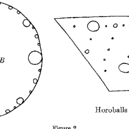
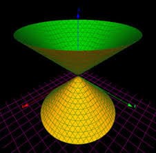
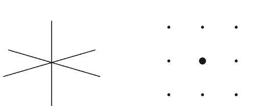
$f_i \in K[x]=K\left[x_1, \ldots, x_n\right]$ and $K$ a field. The solution set is called an algebraic set or algebraic variety. The pictures in Figures A.1 – A.8 show examples of algebraic varieties.
However, algebraic sets really live in different worlds, depending on whether $K$ is algebraically closed or not. For instance, the question whether the simple polynomial equation $x^n+y^n+z^n=0, n \geq 3$, has any non-trivial solution in $K$, is of fundamental difference if we ask this for $K$ to be $\mathbb{C}, \mathbb{R}$ or $\mathbb{Q}$. (For $\mathbb{C}$ we obtain a surface, for $\mathbb{R}$ we obtain a surface if $n$ is odd but only ${0}$ if $n$ is even, and for $\mathbb{Q}$ this is Fermat’s problem, solved by A. Wiles in 1994.) Classical algebraic geometry assumes $K$ to be algebraically closed. Real algebraic geometry is a field in its own and the study of varieties over $\mathbb{Q}$ belongs to arithmetic geometry, a merge of algebraic geometry and number theory. In this appendix we assume $K$ to be algebraically closed.
Many of the problems in algebra, in particular, computer algebra, have a geometric origin. Therefore, we choose an introduction by means of some pictures of algebraic varieties, some of them being used to illustrate subsequent problems.
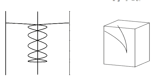
The pictures in this introduction, Figures A.1 – A.8, were not only chosen to illustrate the beauty of algebraic geometric objects but also because these varieties have had some prominent influence on the development of algebraic geometry and singularity theory.
The Clebsch cubic itself has been the object of numerous investigations in global algebraic geometry, the Cayley and the $D_4$-cubic also, but, moreover, since the $D_4$-cubic deforms, via the Cayley cubic, to the Clebsch cubic, these first three pictures illustrate deformation theory, an important branch of (computational) algebraic geometry.
数学代写|交换代数代写Commutative Algebra代考|Affine Algebraic Varieties
From now on, we always assume $K$ to be an algebraically closed field, except when we specify $K$ otherwise.
We start with the simplest algebraic varieties, affine varieties.
Definition A.2.1. $\mathbb{A}^n=\mathbb{A}_K^n$ denotes the $n$-dimensional affine space over $K$, the set of all $n$-tuples $x=\left(x_1, \ldots, x_n\right)$ with $x_i \in K$, together with its structure as affine space.
A set $X \subset \mathbb{A}K^n$ is called an affine algebraic set or a (classical) affine algebraic variety or just an affine variety (over $K$ ) if there exist polynomials $f\lambda \in K\left[x_1, \ldots, x_n\right], \lambda$ in some index set $\Lambda$, such that
$$
X=V\left(\left(f_\lambda\right){\lambda \in \Lambda}\right)=\left{x \in \mathbb{A}_K^n \mid f\lambda(x)=0, \forall \lambda \in \Lambda\right} .
$$
$X$ is then called the zero-set of $\left(f_\lambda\right)_{\lambda \in \Lambda}$.
If $L$ is a non-algebraically closed field and $f_\lambda$ are elements of $L[x]$, we may consider an algebraically closed field $K$ containing $L$ (for example, $K=\bar{L}$, the algebraic closure of $L$ ) and all statements apply to the $f_\lambda$ considered as elements of $K[x]$.
Of course, $X$ depends only on the ideal $I$ generated by the $f_\lambda$, that is, $X=V(I)$ with $I=\left\langle f_\lambda \mid \lambda \in \Lambda\right\rangle_{K[x]}$. By the Hilbert basis theorem, 1.3.5, there are finitely many polynomials such that $I=\left\langle f_1, \ldots, f_k\right\rangle_{K[x]}$ and, hence, $X=V\left(f_1, \ldots, f_k\right)$
If $X=V\left(f_1, \ldots, f_k\right)$ with $\operatorname{deg}\left(f_i\right)=1$, then $X \subset \mathbb{A}^n$ is an affine linear subspace of $\mathbb{A}^n$. If $X=V(f)$ for a single polynomial $f \in K[x] \backslash{0}$ then $X$ is called a hypersurface in $\mathbb{A}^n$. A hypersurface in $\mathbb{A}^2$ is called an (affine) plane curve and a hypersurface in $\mathbb{A}^3$ an affine surface in 3-space. Hypersurfaces in $\mathbb{A}^n$ of degree $2,3,4,5, \ldots$ are called quadrics, cubics, quartics, quintics,
Figure A.11 shows pictures of examples with respective equations. These can be drawn using Singular as indicated in the following example:
SINGULAR Example A.2.2 (surface plot).
ring $r=0,(x, y, z), d p ;$
poly $f=\ldots ;$
LIB”surf.lib”;
plot $(f) ;$
ring $r=0,(x, y, z), d p$;
poly $f=\ldots$;
LIB”surf. .lib”;
$\operatorname{plot}(f)$;
The pictures shown in Figure A.11 give the correct impression that the varieties become more complicated if we increase the degree of the defining polynomial. However, the pictures are real, and it is quite instructive to see how they change if we change the coefficients of terms (in particular the signs). The quintic in Figure A.11 is the Togliatti quintic, which embellishes the cover of this book.
交换代数代写
数学代写|交换代数代写Commutative Algebra代考|Introduction by Pictures
代数几何的基本问题是理解解的集合 $x=\left(x_1, \ldots, x_n\right) \in K^n$ 多项式方程组
$$
f_1\left(x_1, \ldots, x_n\right)=0, \ldots, f_k\left(x_1, \ldots, x_n\right)=0,
$$
$f_i \in K[x]=K\left[x_1, \ldots, x_n\right]$ 和 $K$ 一个领域。解集称为代数集或代数变集。图A.1 – A.8中的图片展示了代数变量的例子。
然而,代数集确实存在于不同的世界,取决于是否 $K$ 是否代数封闭。例如,简单多项式方程是否 $x^n+y^n+z^n=0, n \geq 3$的非平凡解 $K$如果我们要求这样做,就会有根本的区别 $K$ 成为 $\mathbb{C}, \mathbb{R}$ 或 $\mathbb{Q}$. (适用于 $\mathbb{C}$ 我们得到一个曲面 $\mathbb{R}$ 我们得到一个曲面 $n$ 只是奇怪而已 ${0}$ 如果 $n$ 是偶数,和为 $\mathbb{Q}$ 这是费马的问题,1994年由A.怀尔斯解决。)经典代数几何假设 $K$ 代数封闭。真正的代数几何是一个在其自身和变种的研究领域 $\mathbb{Q}$ 属于算术几何,是代数几何和数论的融合。在本附录中,我们假设 $K$ 代数封闭。代数中的许多问题,特别是计算机代数中的许多问题,都有一个几何根源。因此,我们选择了一些代数变量的图片作为介绍,其中一些被用来说明后面的问题。
本导论中的图A.1 – A.8不仅是为了说明代数几何对象的美,而且还因为这些变化对代数几何和奇点理论的发展产生了一些突出的影响。
Clebsch立方本身一直是全球代数几何中许多研究的对象,Cayley和 $D_4$——立方也,但,而且,既然 $D_4$-三次变形,通过Cayley三次,到Clebsch三次,这前三幅图说明了变形理论,(计算)代数几何的一个重要分支。
数学代写|交换代数代写Commutative Algebra代考|Affine Algebraic Varieties
从现在开始,我们总是假设$K$是一个代数闭域,除非我们另行指定$K$。
我们从最简单的代数变量开始,仿射变量。
A.2.1.定义$\mathbb{A}^n=\mathbb{A}K^n$表示$K$上的$n$维仿射空间,所有$n$ -元组$x=\left(x_1, \ldots, x_n\right)$与$x_i \in K$的集合,连同其结构作为仿射空间。 集合$X \subset \mathbb{A}K^n$被称为仿射代数集或(经典)仿射代数变数或仅仅是仿射变数(在$K$上),如果在某些指标集合$\Lambda$中存在多项式$f\lambda \in K\left[x_1, \ldots, x_n\right], \lambda$,使得 $$ X=V\left(\left(f\lambda\right){\lambda \in \Lambda}\right)=\left{x \in \mathbb{A}K^n \mid f\lambda(x)=0, \forall \lambda \in \Lambda\right} . $$ 然后将$X$称为$\left(f\lambda\right){\lambda \in \Lambda}$的零集。 如果$L$是一个非代数闭域,并且$f\lambda$是$L[x]$的元素,我们可以考虑一个包含$L$(例如$K=\bar{L}$, $L$的代数闭包)的代数闭域$K$,并且所有的语句都适用于$f_\lambda$作为$K[x]$的元素。
当然,$X$只依赖于理想的$I$生成的$f_\lambda$,即$X=V(I)$与$I=\left\langle f_\lambda \mid \lambda \in \Lambda\right\rangle_{K[x]}$。根据希尔伯特基定理1.3.5,有有限多个多项式使得$I=\left\langle f_1, \ldots, f_k\right\rangle_{K[x]}$和$X=V\left(f_1, \ldots, f_k\right)$
如果$X=V\left(f_1, \ldots, f_k\right)$与$\operatorname{deg}\left(f_i\right)=1$结合,则$X \subset \mathbb{A}^n$是$\mathbb{A}^n$的仿射线性子空间。如果$X=V(f)$对于单个多项式$f \in K[x] \backslash{0}$,那么$X$被称为$\mathbb{A}^n$中的超曲面。$\mathbb{A}^2$中的超曲面称为(仿射)平面曲线,$\mathbb{A}^3$中的超曲面称为三维仿射曲面。次为$2,3,4,5, \ldots$的$\mathbb{A}^n$超曲面称为二次曲面、三次曲面、四次曲面、五次曲面、
图A.11显示了带有相应方程的示例图片。这些可以用单数表示,如下例所示:
奇异例A.2.2(表面图)。
Ring $r=0,(x, y, z), d p ;$
聚$f=\ldots ;$
LIB”surf.lib”;
剧情$(f) ;$
环$r=0,(x, y, z), d p$;
聚$f=\ldots$;
LIB”surf. . LIB”;
$\operatorname{plot}(f)$;
图A.11所示的图片给出了一个正确的印象,即如果我们增加定义多项式的程度,变量会变得更加复杂。然而,这些图片是真实的,如果我们改变项的系数(特别是符号),看到它们是如何变化的,是很有启发性的。图A.11中的五分图是Togliatti五分图,它点缀在本书的封面上。

数学代写|交换代数代写Commutative Algebra代考 请认准UprivateTA™. UprivateTA™为您的留学生涯保驾护航。
微观经济学代写
微观经济学是主流经济学的一个分支,研究个人和企业在做出有关稀缺资源分配的决策时的行为以及这些个人和企业之间的相互作用。my-assignmentexpert™ 为您的留学生涯保驾护航 在数学Mathematics作业代写方面已经树立了自己的口碑, 保证靠谱, 高质且原创的数学Mathematics代写服务。我们的专家在图论代写Graph Theory代写方面经验极为丰富,各种图论代写Graph Theory相关的作业也就用不着 说。
线性代数代写
线性代数是数学的一个分支,涉及线性方程,如:线性图,如:以及它们在向量空间和通过矩阵的表示。线性代数是几乎所有数学领域的核心。
博弈论代写
现代博弈论始于约翰-冯-诺伊曼(John von Neumann)提出的两人零和博弈中的混合策略均衡的观点及其证明。冯-诺依曼的原始证明使用了关于连续映射到紧凑凸集的布劳威尔定点定理,这成为博弈论和数学经济学的标准方法。在他的论文之后,1944年,他与奥斯卡-莫根斯特恩(Oskar Morgenstern)共同撰写了《游戏和经济行为理论》一书,该书考虑了几个参与者的合作游戏。这本书的第二版提供了预期效用的公理理论,使数理统计学家和经济学家能够处理不确定性下的决策。
微积分代写
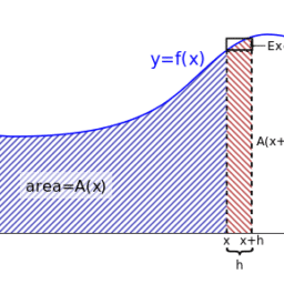
微积分,最初被称为无穷小微积分或 “无穷小的微积分”,是对连续变化的数学研究,就像几何学是对形状的研究,而代数是对算术运算的概括研究一样。
它有两个主要分支,微分和积分;微分涉及瞬时变化率和曲线的斜率,而积分涉及数量的累积,以及曲线下或曲线之间的面积。这两个分支通过微积分的基本定理相互联系,它们利用了无限序列和无限级数收敛到一个明确定义的极限的基本概念 。
计量经济学代写
什么是计量经济学?
计量经济学是统计学和数学模型的定量应用,使用数据来发展理论或测试经济学中的现有假设,并根据历史数据预测未来趋势。它对现实世界的数据进行统计试验,然后将结果与被测试的理论进行比较和对比。
根据你是对测试现有理论感兴趣,还是对利用现有数据在这些观察的基础上提出新的假设感兴趣,计量经济学可以细分为两大类:理论和应用。那些经常从事这种实践的人通常被称为计量经济学家。
Matlab代写
MATLAB 是一种用于技术计算的高性能语言。它将计算、可视化和编程集成在一个易于使用的环境中,其中问题和解决方案以熟悉的数学符号表示。典型用途包括:数学和计算算法开发建模、仿真和原型制作数据分析、探索和可视化科学和工程图形应用程序开发,包括图形用户界面构建MATLAB 是一个交互式系统,其基本数据元素是一个不需要维度的数组。这使您可以解决许多技术计算问题,尤其是那些具有矩阵和向量公式的问题,而只需用 C 或 Fortran 等标量非交互式语言编写程序所需的时间的一小部分。MATLAB 名称代表矩阵实验室。MATLAB 最初的编写目的是提供对由 LINPACK 和 EISPACK 项目开发的矩阵软件的轻松访问,这两个项目共同代表了矩阵计算软件的最新技术。MATLAB 经过多年的发展,得到了许多用户的投入。在大学环境中,它是数学、工程和科学入门和高级课程的标准教学工具。在工业领域,MATLAB 是高效研究、开发和分析的首选工具。MATLAB 具有一系列称为工具箱的特定于应用程序的解决方案。对于大多数 MATLAB 用户来说非常重要,工具箱允许您学习和应用专业技术。工具箱是 MATLAB 函数(M 文件)的综合集合,可扩展 MATLAB 环境以解决特定类别的问题。可用工具箱的领域包括信号处理、控制系统、神经网络、模糊逻辑、小波、仿真等。