MY-ASSIGNMENTEXPERT™可以为您提供sydney FINC6009 Portfolio Theory投资组合课程的代写代考和辅导服务!
这是悉尼大学投资组合课程的代写成功案例。
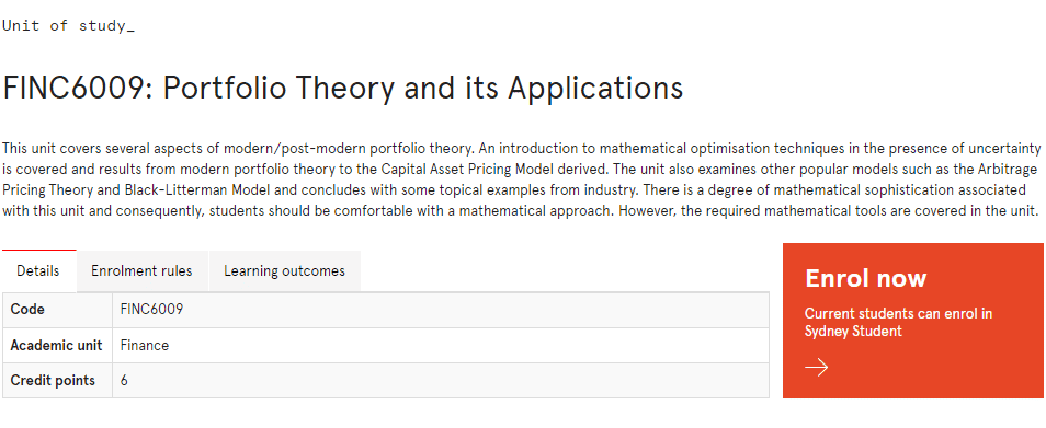
FINC6009课程简介
This unit covers several aspects of modern/post-modern portfolio theory. An introduction to mathematical optimisation techniques in the presence of uncertainty is covered and results from modern portfolio theory to the Capital Asset Pricing Model derived. The unit also examines other popular models such as the Arbitrage Pricing Theory and Black-Litterman Model and concludes with some topical examples from industry. There is a degree of mathematical sophistication associated with this unit and consequently, students should be comfortable with a mathematical approach. However, the required mathematical tools are covered in the unit.
Prerequisites
At the completion of this unit, you should be able to:
- LO1. describe portfolio and investment problems in a mathematical context to enable an advanced approach to portfolio construction.
- LO2. provide a detailed explanation of the mathematical and economic principles of risk and return and demonstrate how that relates to portfolio theory.
- LO3. apply the principles of portfolio theory to solve practical investment problems utilising EXCEL and/or other software packages
- LO4. contrast different approaches to portfolio theory and explain the strengths and weaknesses of the various models covered.
FINC6009 Portfolio Theory HELP(EXAM HELP, ONLINE TUTOR)
From our preceding discussion, rational-risk averse investors in reasonably efficient markets can assess the likely profitability of their corporate investments by a statistical weighting of expected returns. Based on a normal distribution of random variables (the familiar bell-shaped curve):
Investors expect either a maximum return for a given level of risk, or a given return for minimum risk.
Risk is measured by the standard deviation of returns and the overall expected return measured by a weighted probabilistic average.
To illustrate the whole procedure, let us begin simply, by graphing a summary of the risk-return profiles for three prospective projects (A, B and C) presented to a corporate board meeting by their financial Director These projects are mutually exclusive (i.e. the selection of one precludes any other).
The risk-return paradox cannot be resolved by statistical analyses alone. Accept-reject investment criteria also depend on the behavioural attitudes of decision-makers towards different normal curves. In our previous example, corporate management’s perception of project risk (preference, indifference and aversion) relative to returns for projects A and B.
Speculative investors among you may have focussed on the greater upside of returns (albeit with an equal probability of occurrence on their downside) and opted for project B. Others, who are more conservative, may have been swayed by downside limitation and opted for A.
For the moment, suffice it to say that, there is no universally correct answer. Ultimately, investment decisions depend on the current risk attitudes of individuals towards possible future returns, measured by their utility curve. Theoretically, these curves are simple to calibrate, but less so in practice. Individually, utility can vary markedly over time and be unique. There is also the vexed question of group decision making.
In our previous Exercise, whose managerial perception of shareholder risk do we calibrate; that of the CEO, the Finance Director, all Board members, or everybody who contributed to the decision process?
And if so, how do we weight them?
Before we start, it should be emphasised that throughout this chapter’s Exercises and the remainder of the text, we shall use the appropriate equations and their numbering from our bookboon.com companion text (PTFA) for cross-reference.
Portfolio Theory and Financial Analyses, 2010.
For example, if we need to define the portfolio return, correlation coefficient and portfolio standard deviation, we might use the following equations from PTFA:
(1) $\mathrm{R}(\mathrm{P})=x \mathrm{R}(\mathrm{A})+(1-x) \mathrm{R}(\mathrm{B})$
(5) $\operatorname{COR}(\mathrm{A}, \mathrm{B})=\frac{\operatorname{COV}(\mathrm{A}, \mathrm{B})}{\sigma \mathrm{A} \sigma \mathrm{B}}$
(8) $\sigma(\mathrm{P})=\sqrt{ } \operatorname{VAR}(\mathrm{P})=\sqrt{ }\left[x^2 \operatorname{VAR}(\mathrm{A})+(1-x)^2 \operatorname{VAR}(\mathrm{B})+2 x(1-x) \operatorname{COR}(\mathrm{A}, \mathrm{B}) \sigma \mathrm{A} \sigma \mathrm{B}\right]$
So, check these out and all the other equations in Chapter Two of PTA before we proceed. And as we develop or adapt them in future exercises, remember that you can always refer back to the relevant chapter(s) in the companion text.
Irrespective of the correlation coefficient, the previous Exercise explains why risk minimisation represents an objective standard against which management and investors can compare the variance of returns from one portfolio to another. To prove the proposition, you will have observed from Table 3.1 and Figure 3.2 that the decision to place two-thirds of our funds in Project A and one-third in Project B falls between $\mathrm{E}$ and $\mathrm{A}$ when $\operatorname{COR}(\mathrm{A}, \mathrm{B})=0$. This is defined by point 0 along the horizontal line $(-1,0,+1)$, according to the data given in Table 3.1 :
$$
\mathrm{R}(\mathrm{P})=15.98 \%, \sigma(\mathrm{P})=2.83 \%
$$
Because portfolio risk is minimised at point $\mathrm{E}$, with a higher return above and to the left in our diagram, the decision is clearly suboptimal.
At one extreme, speculative investors would place all their funds in Project B at point B hoping to maximise their return (completely oblivious to risk). At the other, the most risk-averse among us would seek out the proportionate investment in A and B which corresponds to E. Between the two, a higher expected return could also be achieved for any degree of risk given by the curve E-A. Thus, all investors would move up to the efficiency frontier E-B and depending upon their attitude toward risk choose an appropriate combination of investments above and to the right of $\mathrm{E}$.
Required:
The mathematically minded among you might wish to confirm that when the correlation coefficient is minus one, but only minus one, risky investments can be combined to construct a riskless portfolio by solving the equation for a portfolio’s standard deviation.
So, let us apply this proposition to the previous data.
An Indicative Outline Solution
We have observed that where a proportion of funds $x$ is invested in Project A and (1-x) in Project B, the portfolio variance can be defined by the familiar equation:
(7) $\operatorname{VAR}(\mathrm{P})=x^2 \operatorname{VAR}(\mathrm{A})+(1-x)^2 \operatorname{VAR}(\mathrm{B})+2 x(1-x) \operatorname{COR}(\mathrm{A}, \mathrm{B}) \sigma \mathrm{A} \sigma \mathrm{B}$
The value of $x$, for which Equation (7) is at a minimum, is given by differentiating VAR(P) with respect to $x$ and setting $\triangle \operatorname{VAR}(\mathrm{P}) / \Delta x=0$, such that:
(17) $x=\frac{\operatorname{VAR}(\mathrm{B})-\operatorname{COR}(\mathrm{A}, \mathrm{B}) \sigma(\mathrm{A}) \sigma(\mathrm{B})}{\operatorname{VAR}(\mathrm{A})+\operatorname{VAR}(\mathrm{B})-2 \operatorname{COR}(\mathrm{A}, \mathrm{B}) \sigma(\mathrm{A}) \sigma(\mathrm{B})}$
Since all the variables in the equation for minimum variance are now known, the risk-return trade-off can be solved. Moreover, if the correlation coefficient equals minus one, risky investments can be combined into a riskless portfolio by solving the following equation when the standard deviation is zero.
(18) $\sigma(\mathrm{P})=\sqrt{ }\left[x^2 \operatorname{VAR}(\mathrm{A})+(1-x)^2 \operatorname{VAR}(\mathrm{B})+2 x(1-x) \operatorname{COR}(\mathrm{A}, \mathrm{B}) \sigma \mathrm{A} \sigma \mathrm{B}\right]=0$
Because this is a quadratic in one unknown $(x)$ it therefore follows that to eliminate portfolio risk when $\operatorname{COR}\mathrm{A}, \mathrm{B}=-1$, the proportion of funds $(x)$ invested in Project A should be:
(19) $x=1-\frac{\sigma(\mathrm{A})}{\sigma(\mathrm{A})+\sigma(\mathrm{B})}$

MY-ASSIGNMENTEXPERT™可以为您提供SYDNEY FINC6009 PORTFOLIO THEORY投资组合课程的代写代考和辅导服务!