MY-ASSIGNMENTEXPERT™可以为您提供iona.edu MTH432 Sampling theory抽样调查课程的代写代考和辅导服务!
这是愛納學院抽样调查课程的代写成功案例。
MTH432课程简介
Syllabus : Principles of sample surveys; Simple, stratified and unequal probability sampling with and without replacement; ratio, product and regression method of estimation, Varying Probability Scheme
An overview of probability and statistics. Experiments; sample spaces; random variables; probability measures and distributions; combinatorics; expectation; data collection and analysis; confidence intervals; selected hypothesis tests.
Lecture
Credits: 3
Prerequisite: MTH 232
Offered in Fall Semester
Prerequisites
Books: You can choose any one of the following book for your reference. Books at serial numbers 1 and 2 are easily available, so I will base my lectures on them. Other books are available in the library.
Sampling Techniques : W.G. Cochran, Wiley (Low price edition available)
Theory and Methods of Survey Sampling : Parimal Mukhopadhyay, Prentice Hall of India
Theory of Sample surveys with applications : P.V. Sukhatme, B.V Sukhatme, S. Sukhatme and C. Asok, IASRI, Delhi
Sampling Methodologies and Applications : P.S.R.S. Rao, Chapman and Hall/ CRC
Sampling Theory and Methods : M.N. Murthy, Statistical Publishing Society, Calcutta (Out of print)
Elements of sampling theory and methods : Z. Govindrajalu, Prentice Hall
Sampling Methods- Exercises and Solutions : Pascal Ardilly and Yves Tille’ (Download here through IITK Library link)
MTH432 Sampling theory HELP(EXAM HELP, ONLINE TUTOR)
The initial rest assupmtion corresponds to a zero-valued auxiliary condition being imposed at a time determined in accordance with the input signal. In this problem we show that if the auxiliary condition used is nonzero or if it is always applied at a fixed time (regardless of the input signal) the corresponding system cannot be LTI. Consider a system whose input $x(t)$ and output $y(t)$ satisfy the first-order differential equation:
$$
\frac{d y(t)}{d t}+2 y(t)=x(t)
$$
(a) Given the auxiliary condition $y(1)=1$, use a counterexample to show that the system is not linear.
(b) Given the auxiliary condition $y(1)=1$, use a counterexample to show that the system is not time invariant.
(c) Given the auxiliary condition $y(1)=1$, show that the system is incrementally linear.
(d) Given the auxiliary condition $y(1)=0$, show that the system is linear but not time invariant.
(e) Given the auxiliary condition $y(0)+y(4)=0$, show that the system is linear but not time invariant.
(a) Consider $x_1(t) \stackrel{S}{\rightarrow} y_1(t)$ and $x_2(t) \stackrel{S}{\rightarrow} y_2(t)$. We know that $y_1(1)=y_2(1)=1$. Now consider a third input to the system which is $x_3(t)=x_1(t)+x_2(t)$. Let the corresponding output be $y_3(t)$. Now, note that $y_3(1)=1 \neq y_1(1)+y_2(1)$. Therefore, the system is not linear. A specific example follows: Consider an input signal $x_1(t)=e^{2 t} u(t)$, the corresponding output for $t>0$ is
$$
y_1(t)=\frac{1}{4} e^{2 t}+A e^{-2 t}
$$
Using the fact that $y_1(1)=1$, we get for $t>0$
$$
y_1(t)=\frac{1}{4} e^{2 t}+\left(1-\frac{e}{4}\right) e^{-2(t-1)}
$$
Now, consider a second signal $x_2(t)=0$. Then, the corresponding output is
$$
y_2(t)=B e^{-2 t}
$$
for $t>0$. Using the fact that $y_2(1)=1$, we get for $t>0$
$$
y_2(t)=e^{-2(t-1)}
$$
Now consider a third signal $x_3(t)=x_1(t)+x_2(t)=x_1(t)$. Note that the output we get still be $y_3(t)=y_1(t)$ for $t>0$. Clearly, $y_3(t) \neq y_1(t)+y_2(t)$ for $t>0$. Therefore, the system is not linear.
(b) Again consider an input signal $x_1(t)=e^{2 t} u(t)$. We know that the corresponding output for $t>0$ with $y_1(1)=1$ is
$$
y_1(t)=\frac{1}{4} e^{2 t}+\left(1-\frac{e}{4}\right) e^{-2(t-1)} .
$$
Now, consider an input signal of the form $x_2(t)=x_1(t-T)=e^{2(t-T)} u(t-T)$. The output for $t>T$ is
$$
y_2(t)=\frac{1}{4} e^{2(t-T)}+A e^{-2 t}
$$
Using the fact that $y_2(1)=1$ and also assuming that $T<1$, we get for $t>T$
$$
y_2(t)=\frac{1}{4} e^{2(t-T)}+\left(1-\frac{1}{4} e^{2(1-T)}\right) e^{-2 t}
$$
Now note that $y_2(t) \neq y_1(t-T)$ for $t>T$. Therefore, the system is not time invariant.
(c) In order to show that system is incrementally linear with the auxiliary condition specified as $y(1)=1$, we need to first show that the system is linear with the axiliary condition specified as $y(1)=0$.
For an input-output pair $x_1(t)$ and $y_1(t)$, we may use (1) and the initial rest condition to write
$$
\frac{d y_1(t)}{d t}+2 y_1(t)=x_1(t), y_1(1)=0
$$
For an input-output pair $x_2(t)$ and $y_2(t)$, we may use (1) and the initial rest condition to write
$$
\frac{d y_2(t)}{d t}+2 y_2(t)=x_2(t), y_2(1)=0
$$
Scaling the first equation by $\alpha$ and second equation by $\beta$ and summing, we get
$$
\left.\frac{d}{d t}\left{\alpha y_1(t)+\beta y_2(t)\right}+2\left{\alpha y_1(t)+\beta y_2(t)\right)\right}=\alpha x_1(t)+\beta x_2(t)
$$
and
$$
y_3(1)=y_1(1)+y_2(1)=0
$$
By inspection, it is clear that the output is $y_3(t)=\alpha y_1(t)+\beta y_2(t)$ when the input is $x_3(t)=\alpha x_1(t)+$ $\beta x_2(t)$. Furthermore, $y_3(1)=0=y_1(1)+y_2(1)$. Therefore, the system is linear.
Therefore, the overall system may be treated as the cascade of a linear system with an adder which adds the response of the system to the auxiliary conditions alone.
(d) In the previous part, we showed that the system is linear when $y(1)=0$. In order to show that the system is not time invariant, consider an input of the form $x_1(t)=e^{2 t} u(t)$. From part (a), we know that the corresponding output will be
$$
y_1(t)=\frac{1}{4} e^{2 t}+A e^{-2 t}
$$
Using the fact that $y_1(1)=0$, we get for $t>0$
$$
y_1(t)=\frac{1}{4} e^{2 t}-\frac{1}{4} e^{-2(t-2)}
$$
Now consider an input of the form $x_2(t)=x_1(t-1 / 2)$. Note that $y_2(1)=0$. Clearly, $y_2(1) \neq$ $y_1(1-1 / 2)=(1 / 4)\left(e-e^3\right)$. Therefore, $y_2(t) \neq y_1(t-1 / 2)$ for all $t$. This implies that the system is not time invariant.
(e) A proof which is similar to the proof for linearity used in part (c) may be used here. We may show that the system is not time invariant by using the method outlined in part (d).
To prove the linearity, we may use the similar method outlined in part (c). For an input-output pair $x_1(t)$ and $y_1(t)$, we may use (1) and the initial rest condition to write
$$
\frac{d y_1(t)}{d t}+2 y_1(t)=x_1(t), y_1(0)+y_1(4)=0
$$
For an input-output pair $x_2(t)$ and $y_2(t)$, we may use (1) and the initial rest condition to write
$$
\frac{d y_2(t)}{d t}+2 y_2(t)=x_2(t), y_2(0)+y_2(4)=0
$$
Scaling the first equation by $\alpha$ and second equation by $\beta$ and summing, we get
$$
\left.\frac{d}{d t}\left{\alpha y_1(t)+\beta y_2(t)\right}+2\left{\alpha y_1(t)+\beta y_2(t)\right)\right}=\alpha x_1(t)+\beta x_2(t)
$$
and
$$
y_3(0)+y_3(4)=y_1(0)+y_1(4)+y_2(0)+y_2(4)=0
$$
By inspection, it is clear that the output is $y_3(t)=\alpha y_1(t)+\beta y_2(t)$ when the input is $x_3(t)=$ $\alpha x_1(t)+\beta x_2(t)$. Furthermore, $y_3(0)+y_3(4)=0=y_1(0)+y_1(4)+y_2(0)+y_2(4)$. Therefore, the system is linear.
To show the system is not time invariant, we again consider an input of the form $x_1(t)=e^{2 t} u(t)$. From part (a), we know that the corresponding output will be
$$
y_1(t)=\frac{1}{4} e^{2 t}+A e^{-2 t}
$$
Using the fact that $y_1(0)+y_1(4)=0$, we get for $t>0$
$$
y_1(t)=\frac{1}{4} e^{2 t}-\frac{1}{4} \cdot \frac{1+e^8}{1+e^{-8}} e^{-2 t}
$$
Now, consider an input signal of the form $x_2(t)=x_1(t-T)=e^{2(t-T)} u(t-T)$. The output for $t>T$,
$$
y_2(t)=\frac{1}{4} e^{2(t-T)}+A e^{-2 t}
$$
Using the fact that $y_2(0)+y_2(4)=0$ and also assuming that $T<1$, we get for $t>T$
$$
y_2(t)=\frac{1}{4} e^{2(t-T)}-\frac{1}{4} \cdot \frac{e^{2(4-T)}+e^{-2 T}}{1+e^{-8}} e^{-2 t} .
$$
Now note that $y_2(t) \neq y_1(t-T)$ for $t>T$. therefore, The system is not time invariant.
Let
$$
x[n]=\left{\begin{array}{ll}
1, & 0 \leq n \leq 9 \
0, & \text { elsewhere }
\end{array} \text { and } h[n]= \begin{cases}1, & 0 \leq n \leq N \
0, & \text { elsewhere }\end{cases}\right.
$$
where $N \leq 9$ is an integer. Determine the value of $N$, given that $y[n]=x[n] * h[n]$ and
$$
y4=5, y14=0
$$
Solution
The signal $y[n]$ is
$$
y[n]=x[n] * h[n]=\sum_{k=-\infty}^{\infty} x[k] h[n-k]
$$
In this case, this summation reduces to
$$
y[n]=\sum_{k=0}^9 x[k] h[n-k]=\sum_{k=0}^9 h[n-k]
$$
From this it is clear that $y[n]$ is a summation of shifted replicas of $h[n]$. Since the last replica will begin at $n=9$ and $h[n]$ is zero for $n>N, y[n]$ is zero for $n>N+9$. Using this and the fact that $y[14]=0$, we may conclude that $N$ can at most be 4 . Furthermore, since $y[4]=5$, we can conclude that $h[n]$ has at least 5 non-zero points. The only value of $N$ which satisfies both these conitions is 4 .
One of the important properties of convolution, in both continuous and discrete time, is the associativity property. In this problem, we will check and illustrate this property.
(a) Prove the equality
$$
[x(t) * h(t)] * g(t)=x(t) *[h(t) * g(t)]
$$
by showing that both sides of (2) equal
$$
\int_{-\infty}^{\infty} \int_{-\infty}^{\infty} x(\tau) h(\delta) g(t-\delta-\tau) d \tau d \delta
$$
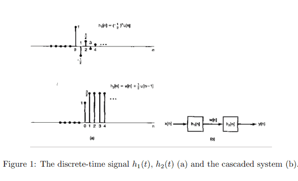
(b) Consider two LTI systems with the unit sample responses $h_1[n]$ and $h_2[n]$ shown in Figure 1 (a). These two systems are cascaded as shown in Figure $1(\mathrm{~b})$. Let $x[n]=u[n]$.
(i) Compute $y[n]$ by first computing $w[n]=x[n] * h_1[n]$ and then computing $y[n]=w[n] * h_2[n]$; that is, $y[n]=\left[x[n] * h_1[n]\right] * h_2[n]$
(ii) Now find $y[n]$ by first convolving $h_1[n]$ and $h_2[n]$ to obtain $g[n]=h_1[n] * h_2[n]$ and then convolving $x[n]$ with $g[n]$ to obtain $y[n]=x[n] *\left(h_1[n] * h_2[n]\right)$.
The answers to (i) and (ii) should be identical, illustrating the associativity property of discrete-time convolution.
(c) Consider the cascade of two LTI system as in Figure 1(b), where in this case
$$
h_1[n]=\sin (8 n)
$$
and
$$
h_2[n]=a^n u[n],|a|<1
$$
and where the input is
$$
x[n]=\delta[n]-a \delta[n-1]
$$
Determine the output $y[n]$. (Hint: The use of the associative and communicative properties of convolution should greatly facilitate the solution.)
Solution
(a) We first have
$$
\begin{aligned}
{[x(t) * h(t)] * g(t) } & =\int_{-\infty}^{\infty} \int_{-\infty}^{\infty} x(\tau) h\left(\delta^{\prime}-\tau\right) g\left(t-\delta^{\prime}\right) d \tau d \delta^{\prime} \
& =\int_{-\infty}^{\infty} \int_{-\infty}^{\infty} x(\tau) h(\delta) g(t-\delta-\tau) d \tau d \delta
\end{aligned}
$$
Also,
$$
\begin{aligned}
x(t) *[h(t) * g(t)] & =\int_{-\infty}^{\infty} \int_{-\infty}^{\infty} x\left(t-\tau^{\prime}\right) h(\tau) g\left(\delta^{\prime}-\tau\right) d \delta^{\prime} d \tau \
& =\int_{-\infty}^{\infty} \int_{-\infty}^{\infty} x(\delta) h(\tau) g(t-\tau-\delta) d \tau d \delta \
& =\int_{-\infty}^{\infty} \int_{-\infty}^{\infty} x(\tau) h(\delta) g(t-\delta-\tau) d \tau d \delta
\end{aligned}
$$
The equality is proved.
(b) (i) We first have
$$
w[n]=u[n] * h_1[n]=\sum_{k=0}^n\left(-\frac{1}{2}\right)^k=\frac{2}{3}\left[1-\left(-\frac{1}{2}\right)^{n+1}\right] u[n]
$$
Now,
$$
y[n]=w[n] * h_2[n]=(n+1) u[n]
$$
(ii) We first have
$$
g[n]=h_1[n] * h_2[n]=\sum_{k=0}^n\left(-\frac{1}{2}\right)^k+\frac{1}{2} \sum_{k=0}^{n-1}\left(-\frac{1}{2}\right)^k=u[n]
$$
Now,
$$
y[n]=u[n] * g[n]=u[n] * u[n]=(n+1) u[n]
$$
The same result was obtained in both parts (i) and (ii).
(c) Note that
$$
x[n] *\left(h_2[n] * h_1[n]\right)=\left(x[n] * h_2[n]\right) * h_1[n] .
$$
Also note that
$$
x[n] * h_2[n]=\alpha^n u[n]-\alpha^n u[n-1]=\delta[n] .
$$
Therefore,
$$
x[n] * h_1[n] * h_2[n]=\delta[n] * \sin (8 n)=\sin (8 n) .
$$

MY-ASSIGNMENTEXPERT™可以为您提供IONA.EDU MTH432 SAMPLING THEORY抽样调查课程的代写代考和辅导服务!。