如果你也在 怎样代写广义相对论General Relativity 这个学科遇到相关的难题,请随时右上角联系我们的24/7代写客服。广义相对论General Relativity又称广义相对论和爱因斯坦引力理论,是爱因斯坦在1915年发表的引力几何理论,是目前现代物理学中对引力的描述。广义相对论概括了狭义相对论并完善了牛顿的万有引力定律,将引力统一描述为空间和时间或四维时空的几何属性。特别是,时空的曲率与任何物质和辐射的能量和动量直接相关。这种关系是由爱因斯坦场方程规定的,这是一个二阶偏微分方程系统。
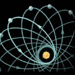
广义相对论General Relativity描述经典引力的牛顿万有引力定律,可以看作是广义相对论对静止质量分布周围几乎平坦的时空几何的预测。然而,广义相对论的一些预言却超出了经典物理学中牛顿的万有引力定律。这些预言涉及时间的流逝、空间的几何、自由落体的运动和光的传播,包括引力时间膨胀、引力透镜、光的引力红移、夏皮罗时间延迟和奇点/黑洞。到目前为止,对广义相对论的所有测试都被证明与该理论一致。广义相对论的时间相关解使我们能够谈论宇宙的历史,并为宇宙学提供了现代框架,从而导致了大爆炸和宇宙微波背景辐射的发现。尽管引入了一些替代理论,广义相对论仍然是与实验数据一致的最简单的理论。然而,广义相对论与量子物理学定律的协调仍然是一个问题,因为缺乏一个自洽的量子引力理论;以及引力如何与三种非引力–强、弱和电磁力统一起来。
广义相对论General Relativity代写,免费提交作业要求, 满意后付款,成绩80\%以下全额退款,安全省心无顾虑。专业硕 博写手团队,所有订单可靠准时,保证 100% 原创。最高质量的广义相对论General Relativity作业代写,服务覆盖北美、欧洲、澳洲等 国家。 在代写价格方面,考虑到同学们的经济条件,在保障代写质量的前提下,我们为客户提供最合理的价格。 由于作业种类很多,同时其中的大部分作业在字数上都没有具体要求,因此广义相对论General Relativity作业代写的价格不固定。通常在专家查看完作业要求之后会给出报价。作业难度和截止日期对价格也有很大的影响。
同学们在留学期间,都对各式各样的作业考试很是头疼,如果你无从下手,不如考虑my-assignmentexpert™!
my-assignmentexpert™提供最专业的一站式服务:Essay代写,Dissertation代写,Assignment代写,Paper代写,Proposal代写,Proposal代写,Literature Review代写,Online Course,Exam代考等等。my-assignmentexpert™专注为留学生提供Essay代写服务,拥有各个专业的博硕教师团队帮您代写,免费修改及辅导,保证成果完成的效率和质量。同时有多家检测平台帐号,包括Turnitin高级账户,检测论文不会留痕,写好后检测修改,放心可靠,经得起任何考验!
想知道您作业确定的价格吗? 免费下单以相关学科的专家能了解具体的要求之后在1-3个小时就提出价格。专家的 报价比上列的价格能便宜好几倍。
我们在物理Physical代写方面已经树立了自己的口碑, 保证靠谱, 高质且原创的物理Physical代写服务。我们的专家在广义相对论General Relativity代写方面经验极为丰富,各种广义相对论General Relativity相关的作业也就用不着说。
物理代写|广义相对论代写General Relativity代考|Differentiable Manifolds
We will begin by briefly defining an $N$-dimensional differentiable manifold $M$. (See $[23,38,56,130]$.) There are a few assumptions in this definition. A set with a topology is one in which open subsets are known. Furthermore, if for every two distinct elements (or points) $p$ and $q$ there exist open and disjoint subsets containing $p$ and $q$, respectively, then the topology is called Hausdorff. A connected Hausdorff manifold is paracompact if and only if it has a countable basis of open sets. (See [1, $130,132]$.
The first assumption we make about an applicable differentiable manifold $M$ is that it is endowed with a paracompact topology.
(Remark: This assumption is necessary for the purpose of integration in any domain.)
We also consider only a connected set $M$ for physical reasons. Moreover, we mostly deal with situations where $M$ is an open set.
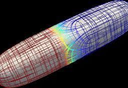
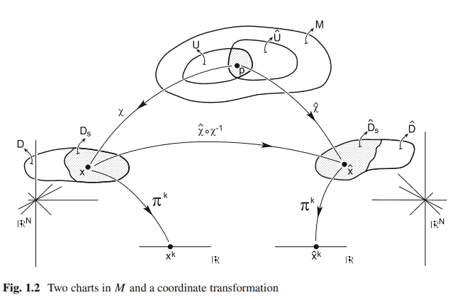
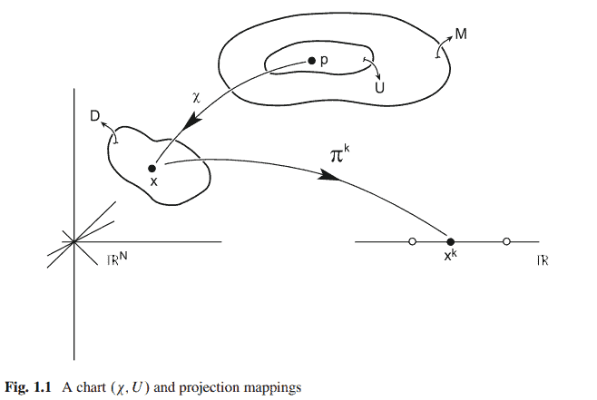
Now we shall introduce local coordinates for $M$. A chart $(\chi, U)$ or a local coordinate system is a pair consisting of an open subset $U \subset M$ together with a continuous, one-to-one mapping (homeomorphism) $\chi$ from $U$ into (codomain) $D \subset \mathbb{R}^N$. Here, $D$ is an open subset of $\mathbb{R}^N$ with the usual Euclidean topology. ${ }^1$ For a point $p \in M$, we have $x \equiv\left(x^1, x^2, \ldots, x^N\right)=\chi(p) \in D$. The coordinates $\left(x^1, x^2, \ldots, x^N\right)$ are the coordinates of the point $p$ in the chart $(\chi, U)$.
Each of the $N$ coordinates is obtained by the projection mappings $\pi^k: D \subset$ $\mathbb{R}^N \longrightarrow \mathbb{R}, k \in{1, \ldots, N}$. These are defined by $\pi^k(x) \equiv \pi^k\left(x^1, \ldots, x^N\right)=$ : $x^k \in \mathbb{R}$. (See Fig. 1.1.)
By the first assumption of paracompactness, we can conclude $[38,130]$ that open subsets $U_h$ exist $^2$ such that $M=\bigcup_h U_h$. The second assumption about $M$ is the following:
There exist countable charts $\left(\chi_h, U_h\right)$ for $M$. Moreover, wherever there is a nonempty intersection between charts, coordinate transformations as in (1.2) of class $C^r$ can be found.
Such a basis of charts for $M$ is called a $C^r$-Atlas. A maximal collection of $C^r$ related atlases is called a maximal $C^r$-Atlas. (It is also called the complete atlas.) Finally, we are in a position to define a differentiable manifold.
An $N$-dimensional $C^r$-differentiable manifold is a set $M$ with a maximal $C^r$ atlas.
物理代写|广义相对论代写General Relativity代考|Tensor Fields Over Differentiable Manifolds
The linear combination of two mixed tensors are defined by:
$$
\begin{aligned}
& {\left[\lambda{ }s^r \mathbf{T}{x_0}+\mu{ }s^r \mathbf{W}{x_0}\right]\left(\tilde{\mathbf{u}}{x_0}^1, \ldots, \tilde{\mathbf{u}}{x_0}^r ; \overrightarrow{\mathbf{a}}{1 x_0}, \ldots, \overrightarrow{\mathbf{a}}{s x_0}\right) } \
&:= \lambda\left[{ }s^r \mathbf{T}{x_0}\left(\tilde{\mathbf{u}}{x_0}^1, \ldots, \tilde{\mathbf{u}}{x_0}^r ; \overrightarrow{\mathbf{a}}{1 x_0}, \ldots, \overrightarrow{\mathbf{a}}{s x_0}\right)\right] \
&+\mu\left[{ }s^r \mathbf{W}{x_0}\left(\tilde{\mathbf{u}}{x_0}^1, \ldots, \tilde{\mathbf{u}}{x_0}^r ; \overrightarrow{\mathbf{a}}{1 x_0}, \ldots, \overrightarrow{\mathbf{a}}{s x_0}\right)\right]
\end{aligned}
$$
for all $\lambda, \mu$ in $\mathbb{R}$, all $\tilde{\mathbf{u}}{x_0}^1, \ldots, \tilde{\mathbf{u}}{x_0}^r$ in $\tilde{\mathbf{T}}{x_0}\left(\mathbb{R}^N\right)$ and all $\overrightarrow{\mathbf{a}}{1 x_0}, \ldots, \overrightarrow{\mathbf{a}}{s x_0}$ in $\mathbf{T}{x_0}\left(\mathbb{R}^N\right)$. (Note that addition between two tensors of different order is not permitted.)
It can be proved via (1.27) that the set of all mixed tensors of order $(r+s)$ constitutes a (real) vector space of dimension $N^{r+s}$.
The tensor product (or outer product) between two tensors ${ }{s_0}^{r{x_0}}$ and ${ }q^p \mathbf{W}{x_0}$ is defined by the function ${ }s^r \mathbf{T}{x_0} \otimes{ }q^p \mathbf{W}{x_0}$ from $\underbrace{\tilde{T}{x_0}\left(\mathbb{R}^N\right) \times \cdots \times \tilde{T}{x_0}\left(\mathbb{R}^N\right)}{r+p}$ $\times \underbrace{T{x_0}\left(\mathbb{R}^N\right) \times \cdots \times T_{x_0}\left(\mathbb{R}^{\mathbb{N}}\right)}{s+q}$ into $\mathbb{R}$ such that $$ \begin{aligned} & {\left[{ }_s^r \mathbf{T}{x_0}\right.}\left.\otimes{ }q^p \mathbf{W}{x_0}\right]\left(\tilde{\mathbf{u}}{x_0}^1, \ldots, \tilde{\mathbf{u}}{x_0}^r ; \tilde{\mathbf{v}}{x_0}^1, \ldots, \tilde{\mathbf{v}}{x_0}^p ; \overrightarrow{\mathbf{a}}{1 x_0}, \ldots, \overrightarrow{\mathbf{a}}{s x_0} ; \overrightarrow{\mathbf{b}}{1 x_0}, \ldots, \overrightarrow{\mathbf{b}}{q x_0}\right) \
& \quad=:\left[{ }s^r \mathbf{T}{x_0}\left(\tilde{\mathbf{u}}{x_0}^1, \ldots, \tilde{\mathbf{u}}{x_0}^r ; \overrightarrow{\mathbf{a}}{1 x_0}, \ldots, \overrightarrow{\mathbf{a}}{s x_0}\right)\right] \times\left[{ }q^p \mathbf{W}{x_0}\left(\tilde{\mathbf{v}}{x_0}^1, \ldots, \tilde{\mathbf{v}}{x_0}^p ; \overrightarrow{\mathbf{b}}{1 x_0}, \ldots, \overrightarrow{\mathbf{b}}{q x_0}\right)\right]
\end{aligned}
$$
for all $\overrightarrow{\mathbf{a}}{1 x_0}, \ldots, \overrightarrow{\mathbf{a}}{s x_0} ; \overrightarrow{\mathbf{b}}{1 x_0}, \ldots, \overrightarrow{\mathbf{b}}{q x_0}$ in $T_{x_0}\left(\mathbb{R}^N\right)$ and all $\tilde{\mathbf{u}}{x_0}^1, \ldots, \tilde{\mathbf{u}}{x_0}^r ; \tilde{\mathbf{v}}{x_0}^1, \ldots$, $\tilde{\mathbf{v}}{x_0}^p$ in $\tilde{T}{x_0}\left(\mathbb{R}^N\right)$. Note that ${ }_s^r \mathbf{T}{x_0} \otimes{ }q^p \mathbf{W}{x_0}$ is a tensor of order $(r+p)+(s+q)$.
Example 1.2.3. Let $N=2$ and $\left{\overrightarrow{\mathbf{e}}{1 x_0}, \overrightarrow{\mathbf{e}}{2 x_0}\right}$ be a basis set for $T_{x_0}\left(\mathbb{R}^N\right)$. Let two covariant tensors, ${ }1^0 \mathbf{T}{x_0}$ and ${ }2^0 \mathbf{W}{x_0}$, be defined by
$$
\begin{aligned}
& \overrightarrow{\mathbf{a}}{x_0}=\alpha^1 \overrightarrow{\mathbf{e}}{1 x_0}+\alpha^2 \overrightarrow{\mathbf{e}}{2 x_0}, \overrightarrow{\mathbf{b}}{1 x_0}=\beta_1^1 \overrightarrow{\mathbf{e}}{1 x_0}+\beta_1^2 \overrightarrow{\mathbf{e}}{2 x_0}, \overrightarrow{\mathbf{b}}{2 x_0}=\beta_2^1 \overrightarrow{\mathbf{e}}{1 x_0}+\beta_2^2 \overrightarrow{\mathbf{e}}{2 x_0}, \ & \overrightarrow{\mathbf{c}}{x_0}=\gamma^1 \overrightarrow{\mathbf{e}}{1 x_0}+\gamma^2 \overrightarrow{\mathbf{e}}{2 x_0} ; \
& { }1^0 \mathbf{T}{x_0}\left(\overrightarrow{\mathbf{a}}{x_0}\right):=\alpha^1, \quad{ }_2^0 \mathbf{W}{x_0}\left(\overrightarrow{\mathbf{b}}{1 x_0}, \overrightarrow{\mathbf{b}}{2 x_0}\right):=\beta_1^1 \beta_2^2 .
\end{aligned}
$$
广义相对论代写
物理代写|广义相对论代写General Relativity代考|Differentiable Manifolds
我们首先简单地定义一个$N$维可微流形$M$。(参见$[23,38,56,130]$。)在这个定义中有一些假设。具有拓扑的集合是其中开放子集已知的集合。更进一步,如果对于每两个不同的元素(或点)$p$和$q$,分别存在包含$p$和$q$的开放和不相交子集,则该拓扑称为Hausdorff。连通的Hausdorff流形是准紧的当且仅当它具有开集的可数基。(参见[1,$130,132]$]。
对于一个适用的可微流形$M$,我们的第一个假设是它具有一个准紧拓扑。
(注:这个假设对于任何领域的集成都是必要的。)
由于物理原因,我们也只考虑连通集$M$。此外,我们主要处理$M$是开放集的情况。
现在我们将引入$M$的局部坐标。图表$(\chi, U)$或局部坐标系是由开放子集$U \subset M$和从$U$到(上域)$D \subset \mathbb{R}^N$的连续的、一对一的映射(同胚)$\chi$组成的一对。这里,$D$是$\mathbb{R}^N$的开放子集,具有通常的欧几里得拓扑结构。${ }^1$对于点$p \in M$,我们有$x \equiv\left(x^1, x^2, \ldots, x^N\right)=\chi(p) \in D$。坐标$\left(x^1, x^2, \ldots, x^N\right)$是图表$(\chi, U)$中点$p$的坐标。
每个$N$坐标都是通过投影映射$\pi^k: D \subset$$\mathbb{R}^N \longrightarrow \mathbb{R}, k \in{1, \ldots, N}$获得的。它们由$\pi^k(x) \equiv \pi^k\left(x^1, \ldots, x^N\right)=$: $x^k \in \mathbb{R}$定义。(见图1.1)
通过准紧性的第一个假设,我们可以得出$[38,130]$开放子集$U_h$存在$^2$使得$M=\bigcup_h U_h$。关于$M$的第二个假设如下:
对于$M$,存在可数的图表$\left(\chi_h, U_h\right)$。此外,只要图表之间存在非空相交,就可以找到类$C^r$(1.2)中的坐标转换。
这种$M$的基本图表被称为$C^r$ -Atlas。$C^r$相关地图集的最大集合称为最大$C^r$ -地图集。(它也被称为完整地图集。)最后,我们可以定义一个可微流形。
一个$N$维的$C^r$ -可微流形是一个集$M$与一个极大的$C^r$图集。
物理代写|广义相对论代写General Relativity代考|Tensor Fields Over Differentiable Manifolds
两个混合张量的线性组合定义为:
$$
\begin{aligned}
& {\left[\lambda{ }s^r \mathbf{T}{x_0}+\mu{ }s^r \mathbf{W}{x_0}\right]\left(\tilde{\mathbf{u}}{x_0}^1, \ldots, \tilde{\mathbf{u}}{x_0}^r ; \overrightarrow{\mathbf{a}}{1 x_0}, \ldots, \overrightarrow{\mathbf{a}}{s x_0}\right) } \
&:= \lambda\left[{ }s^r \mathbf{T}{x_0}\left(\tilde{\mathbf{u}}{x_0}^1, \ldots, \tilde{\mathbf{u}}{x_0}^r ; \overrightarrow{\mathbf{a}}{1 x_0}, \ldots, \overrightarrow{\mathbf{a}}{s x_0}\right)\right] \
&+\mu\left[{ }s^r \mathbf{W}{x_0}\left(\tilde{\mathbf{u}}{x_0}^1, \ldots, \tilde{\mathbf{u}}{x_0}^r ; \overrightarrow{\mathbf{a}}{1 x_0}, \ldots, \overrightarrow{\mathbf{a}}{s x_0}\right)\right]
\end{aligned}
$$
对于$\mathbb{R}$中的所有$\lambda, \mu$, $\tilde{\mathbf{T}}{x_0}\left(\mathbb{R}^N\right)$中的所有$\tilde{\mathbf{u}}{x_0}^1, \ldots, \tilde{\mathbf{u}}{x_0}^r$和$\mathbf{T}{x_0}\left(\mathbb{R}^N\right)$中的所有$\overrightarrow{\mathbf{a}}{1 x_0}, \ldots, \overrightarrow{\mathbf{a}}{s x_0}$。(注意两个不同阶张量之间的加法是不允许的。)
由式(1.27)可以证明,所有阶为$(r+s)$的混合张量的集合构成一个维数为$N^{r+s}$的(实)向量空间。
两个张量${ }{s_0}^{r{x_0}}$和${ }q^p \mathbf{W}{x_0}$之间的张量积(或外积)由${ }s^r \mathbf{T}{x_0} \otimes{ }q^p \mathbf{W}{x_0}$函数定义,从$\underbrace{\tilde{T}{x_0}\left(\mathbb{R}^N\right) \times \cdots \times \tilde{T}{x_0}\left(\mathbb{R}^N\right)}{r+p}$$\times \underbrace{T{x_0}\left(\mathbb{R}^N\right) \times \cdots \times T_{x_0}\left(\mathbb{R}^{\mathbb{N}}\right)}{s+q}$到$\mathbb{R}$,使得$$ \begin{aligned} & {\left[{ }s^r \mathbf{T}{x_0}\right.}\left.\otimes{ }q^p \mathbf{W}{x_0}\right]\left(\tilde{\mathbf{u}}{x_0}^1, \ldots, \tilde{\mathbf{u}}{x_0}^r ; \tilde{\mathbf{v}}{x_0}^1, \ldots, \tilde{\mathbf{v}}{x_0}^p ; \overrightarrow{\mathbf{a}}{1 x_0}, \ldots, \overrightarrow{\mathbf{a}}{s x_0} ; \overrightarrow{\mathbf{b}}{1 x_0}, \ldots, \overrightarrow{\mathbf{b}}{q x_0}\right) \ & \quad=:\left[{ }s^r \mathbf{T}{x_0}\left(\tilde{\mathbf{u}}{x_0}^1, \ldots, \tilde{\mathbf{u}}{x_0}^r ; \overrightarrow{\mathbf{a}}{1 x_0}, \ldots, \overrightarrow{\mathbf{a}}{s x_0}\right)\right] \times\left[{ }q^p \mathbf{W}{x_0}\left(\tilde{\mathbf{v}}{x_0}^1, \ldots, \tilde{\mathbf{v}}{x_0}^p ; \overrightarrow{\mathbf{b}}{1 x_0}, \ldots, \overrightarrow{\mathbf{b}}{q x_0}\right)\right] \end{aligned} $$ 对于$T{x_0}\left(\mathbb{R}^N\right)$中的所有$\overrightarrow{\mathbf{a}}{1 x_0}, \ldots, \overrightarrow{\mathbf{a}}{s x_0} ; \overrightarrow{\mathbf{b}}{1 x_0}, \ldots, \overrightarrow{\mathbf{b}}{q x_0}$和$\tilde{T}{x_0}\left(\mathbb{R}^N\right)$中的所有$\tilde{\mathbf{u}}{x_0}^1, \ldots, \tilde{\mathbf{u}}{x_0}^r ; \tilde{\mathbf{v}}{x_0}^1, \ldots$, $\tilde{\mathbf{v}}{x_0}^p$。注意${ }s^r \mathbf{T}{x_0} \otimes{ }q^p \mathbf{W}{x_0}$是一个$(r+p)+(s+q)$阶张量。 例1.2.3。设$N=2$和$\left{\overrightarrow{\mathbf{e}}{1 x_0}, \overrightarrow{\mathbf{e}}{2 x_0}\right}$为$T{x_0}\left(\mathbb{R}^N\right)$的基集。设两个协变张量${ }1^0 \mathbf{T}{x_0}$和${ }2^0 \mathbf{W}{x_0}$,定义为
$$
\begin{aligned}
& \overrightarrow{\mathbf{a}}{x_0}=\alpha^1 \overrightarrow{\mathbf{e}}{1 x_0}+\alpha^2 \overrightarrow{\mathbf{e}}{2 x_0}, \overrightarrow{\mathbf{b}}{1 x_0}=\beta_1^1 \overrightarrow{\mathbf{e}}{1 x_0}+\beta_1^2 \overrightarrow{\mathbf{e}}{2 x_0}, \overrightarrow{\mathbf{b}}{2 x_0}=\beta_2^1 \overrightarrow{\mathbf{e}}{1 x_0}+\beta_2^2 \overrightarrow{\mathbf{e}}{2 x_0}, \ & \overrightarrow{\mathbf{c}}{x_0}=\gamma^1 \overrightarrow{\mathbf{e}}{1 x_0}+\gamma^2 \overrightarrow{\mathbf{e}}{2 x_0} ; \
& { }1^0 \mathbf{T}{x_0}\left(\overrightarrow{\mathbf{a}}{x_0}\right):=\alpha^1, \quad{ }_2^0 \mathbf{W}{x_0}\left(\overrightarrow{\mathbf{b}}{1 x_0}, \overrightarrow{\mathbf{b}}{2 x_0}\right):=\beta_1^1 \beta_2^2 .
\end{aligned}
$$

物理代写|广义相对论代写General Relativity代考 请认准UprivateTA™. UprivateTA™为您的留学生涯保驾护航。
微观经济学代写
微观经济学是主流经济学的一个分支,研究个人和企业在做出有关稀缺资源分配的决策时的行为以及这些个人和企业之间的相互作用。my-assignmentexpert™ 为您的留学生涯保驾护航 在数学Mathematics作业代写方面已经树立了自己的口碑, 保证靠谱, 高质且原创的数学Mathematics代写服务。我们的专家在图论代写Graph Theory代写方面经验极为丰富,各种图论代写Graph Theory相关的作业也就用不着 说。
线性代数代写
线性代数是数学的一个分支,涉及线性方程,如:线性图,如:以及它们在向量空间和通过矩阵的表示。线性代数是几乎所有数学领域的核心。
博弈论代写
现代博弈论始于约翰-冯-诺伊曼(John von Neumann)提出的两人零和博弈中的混合策略均衡的观点及其证明。冯-诺依曼的原始证明使用了关于连续映射到紧凑凸集的布劳威尔定点定理,这成为博弈论和数学经济学的标准方法。在他的论文之后,1944年,他与奥斯卡-莫根斯特恩(Oskar Morgenstern)共同撰写了《游戏和经济行为理论》一书,该书考虑了几个参与者的合作游戏。这本书的第二版提供了预期效用的公理理论,使数理统计学家和经济学家能够处理不确定性下的决策。
微积分代写
微积分,最初被称为无穷小微积分或 “无穷小的微积分”,是对连续变化的数学研究,就像几何学是对形状的研究,而代数是对算术运算的概括研究一样。
它有两个主要分支,微分和积分;微分涉及瞬时变化率和曲线的斜率,而积分涉及数量的累积,以及曲线下或曲线之间的面积。这两个分支通过微积分的基本定理相互联系,它们利用了无限序列和无限级数收敛到一个明确定义的极限的基本概念 。
计量经济学代写
什么是计量经济学?
计量经济学是统计学和数学模型的定量应用,使用数据来发展理论或测试经济学中的现有假设,并根据历史数据预测未来趋势。它对现实世界的数据进行统计试验,然后将结果与被测试的理论进行比较和对比。
根据你是对测试现有理论感兴趣,还是对利用现有数据在这些观察的基础上提出新的假设感兴趣,计量经济学可以细分为两大类:理论和应用。那些经常从事这种实践的人通常被称为计量经济学家。
Matlab代写
MATLAB 是一种用于技术计算的高性能语言。它将计算、可视化和编程集成在一个易于使用的环境中,其中问题和解决方案以熟悉的数学符号表示。典型用途包括:数学和计算算法开发建模、仿真和原型制作数据分析、探索和可视化科学和工程图形应用程序开发,包括图形用户界面构建MATLAB 是一个交互式系统,其基本数据元素是一个不需要维度的数组。这使您可以解决许多技术计算问题,尤其是那些具有矩阵和向量公式的问题,而只需用 C 或 Fortran 等标量非交互式语言编写程序所需的时间的一小部分。MATLAB 名称代表矩阵实验室。MATLAB 最初的编写目的是提供对由 LINPACK 和 EISPACK 项目开发的矩阵软件的轻松访问,这两个项目共同代表了矩阵计算软件的最新技术。MATLAB 经过多年的发展,得到了许多用户的投入。在大学环境中,它是数学、工程和科学入门和高级课程的标准教学工具。在工业领域,MATLAB 是高效研究、开发和分析的首选工具。MATLAB 具有一系列称为工具箱的特定于应用程序的解决方案。对于大多数 MATLAB 用户来说非常重要,工具箱允许您学习和应用专业技术。工具箱是 MATLAB 函数(M 文件)的综合集合,可扩展 MATLAB 环境以解决特定类别的问题。可用工具箱的领域包括信号处理、控制系统、神经网络、模糊逻辑、小波、仿真等。