如果你也在 怎样代写量子场论Quantum field theory 这个学科遇到相关的难题,请随时右上角联系我们的24/7代写客服。商量子场论Quantum field theory是经典场论、量子力学和狭义相对论结合的结果。最早成功的经典场论是由牛顿的万有引力定律产生的,尽管在他1687年的论文《Philosophiæ Naturalis Principia Mathematica》中完全没有场的概念。牛顿所描述的引力是一种 “远距离作用”–它对远处物体的影响是瞬间的,无论距离多远。
量子场论Quantum field theory通过博恩、海森堡和帕斯卡尔-乔丹在1925-1926年的工作,自由电磁场(没有与物质相互作用的电磁场)的量子理论通过经典量子化被开发出来,将电磁场视为一组量子谐波振荡器。 然而,由于排除了相互作用,这样的理论还不能对现实世界作出定量预测。
my-assignmentexpert™量子场论Quantum field theory代写,免费提交作业要求, 满意后付款,成绩80\%以下全额退款,安全省心无顾虑。专业硕 博写手团队,所有订单可靠准时,保证 100% 原创。my-assignmentexpert™, 最高质量的量子场论Quantum field theory作业代写,服务覆盖北美、欧洲、澳洲等 国家。 在代写价格方面,考虑到同学们的经济条件,在保障代写质量的前提下,我们为客户提供最合理的价格。 由于作业种类很多,同时其中的大部分作业在字数上都没有具体要求,因此量子场论Quantum field theory作业代写的价格不固定。通常在经济学专家查看完作业要求之后会给出报价。作业难度和截止日期对价格也有很大的影响。
想知道您作业确定的价格吗? 免费下单以相关学科的专家能了解具体的要求之后在1-3个小时就提出价格。专家的 报价比上列的价格能便宜好几倍。
my-assignmentexpert™ 为您的留学生涯保驾护航 在澳洲代写方面已经树立了自己的口碑, 保证靠谱, 高质且原创的澳洲代写服务。我们的专家在量子场论Quantum field theory代写方面经验极为丰富,各种量子场论Quantum field theory相关的作业也就用不着 说。
我们提供的量子场论Quantum field theory及其相关学科的代写,服务范围广, 其中包括但不限于:

物理代考|量子场论代考Quantum field theory代考|Early infinities
Historically, one of the first confusions about the second-quantized photon field was that the Hamiltonian
$$
H=\int \frac{d^3 k}{(2 \pi)^3} \omega_k\left(a_k^{\dagger} a_k+\frac{1}{2}\right)
$$
with $\omega_k=|\vec{k}|$ seemed to imply that the vacuum has infinite energy,
$$
E_0=\langle 0|H| 0\rangle=\frac{1}{2} \int \frac{d^3 k}{(2 \pi)^3}|\vec{k}|=\infty .
$$
Fortunately, there is an easy way out of this paradoxical infinity: How do you measure the energy of the vacuum? You do not! Only energy differences are measurable, and in these differences the zero-point energy, the energy of the ground state, drops out. This is the basic idea behind renormalization – infinities can appear in intermediate calculations,but they must drop out of physical observables. This zero-point energy does have consequences, such as the Casimir effect (Chapter 15), which comes from the difference in zero-point energies in different size boxes, and the cosmological constant problem, which comes from the fact that energy gravitates. We will come to understand these two examples in detail in Part III, but it makes more sense to start with some less exotic physics.
In 1930, Oppenheimer thought to use perturbation theory to compute the shift of the energy of the hydrogen atom due to the photons [Oppenheimer, 1930]. He got infinity and concluded that QED was wrong. In fact, the result is not infinite but a finite calculable quantity known as the Lamb shift, which agrees perfectly with data. However, it is instructive to understand Oppenheimer’s argument.
物理代考|量子场论代考Quantum field theory代考|Oppenheimer and the Lamb shift
Using OFPT we would calculate the energy shift using
$$
\Delta E_n=\left\langle\psi_n\left|H_{\mathrm{int}}\right| \psi_n\right\rangle+\sum_{m \neq n} \frac{\left|\left\langle\psi_n\left|H_{\mathrm{int}}\right| \psi_m\right\rangle\right|^2}{E_n-E_m} .
$$
This is the standard formula from time-independent perturbation theory. The basic problem is that we have to sum over all possible intermediate states $\left|\psi_m\right\rangle$, including ones that have nothing much to do with the system of interest (for example, free plane waves). It is still true in field theory that there are only a finite number of states below any given energy level $E$, so that as $E \rightarrow \infty, \frac{1}{E-E_n} \rightarrow 0$. The catch is that there are an infinite number of states, and their phase space density goes as $\int d^3 k \sim E^3$, so that you get $\frac{E^3}{E-E_n} \rightarrow \infty$ and perturbation theory breaks down. This is exactly what Oppenheimer found.
First, take something where the calculation makes sense, such as a fixed non-dynamical background field. Say there is an electric field in the $\hat{z}$ direction. Then the potential energy is proportional to the electric field:
$$
H_{\text {int }}=e \vec{E} \cdot \vec{x}=e|E| z .
$$
This interaction produces the linear Stark effect, which is a straightforward application of time-independent perturbation theory in quantum mechanics. Our discussion of the Stark effect here will be limited to a quick demonstration that it is finite, and a representation of the result in terms of diagrams.
Since an atom has no electric dipole moment, the first-order correction is zero:
$$
\left\langle\psi_n\left|H_{\mathrm{int}}\right| \psi_n\right\rangle=0
$$
At second order:
$$
\Delta E_0=\sum_{m>0} \frac{\left|\left\langle\psi_0\left|H_{\text {int }}\right| \psi_m\right\rangle\right|^2}{E_0-E_m}=\overline{\text { 幺 }} \text { 幺े } .
$$
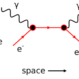
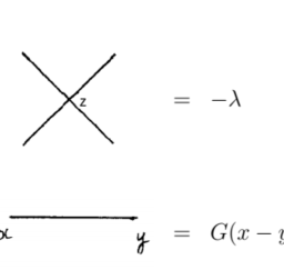
The picture on the right side of this equation is the corresponding Feynman diagram: the 三 symbols represent the electric field which sources photons that interact with the electron (more general background-field calculations will be discussed in Chapters 33 and 34); the electron is represented as the solid line on the bottom; the points where the photon meets the electron correspond to matrix elements of $H_{\mathrm{int}}$; finally, the line between the two photon insertions is the electron propagator, the $\frac{1}{E_0-E_m}$ factor in the second-order expression for $\Delta E_0$.
To show that $\Delta E_0$ is finite, we assume that $E_0<0$ without loss of generality and that $E_m>E_1>E_0$ so that $E_0$ is the ground state. Since $\Delta E_0<0$, by Eq. (4.37), we need to show that $\Delta E_0$ is bounded from below. Using the completeness relation $$ \mathbb{1}=\sum_{m \geq 0}\left|\psi_m\right\rangle\left\langle\psi_m|=| \psi_0\right\rangle\left\langle\psi_0\left|+\sum_{m>0}\right| \psi_m\right\rangle\left\langle\psi_m\right|,
$$
we have
$$
\begin{aligned}
-\Delta E_0 & \leq \frac{1}{E_1-E_0} \sum_{m>0}\left\langle\psi_0\left|H_{\mathrm{int}}\right| \psi_m\right\rangle\left\langle\psi_m\left|H_{\mathrm{int}}\right| \psi_0\right\rangle \
& =\frac{1}{E_1-E_0}\left[\left\langle\psi_0\left|H_{\mathrm{int}}^2\right| \psi_0\right\rangle-\left\langle\psi_0\left|H_{\mathrm{int}}\right| \psi_0\right\rangle^2\right] .
\end{aligned}
$$
量子场论代考
物理代考|量子场论代考Quantum field theory代考|Early infinities
历史上,关于第二量子化光子场的第一个困惑是哈密顿量
$$
H=\int \frac{d^3 k}{(2 \pi)^3} \omega_k\left(a_k^{\dagger} a_k+\frac{1}{2}\right)
$$
$\omega_k=|\vec{k}|$似乎暗示了真空有无限的能量,
$$
E_0=\langle 0|H| 0\rangle=\frac{1}{2} \int \frac{d^3 k}{(2 \pi)^3}|\vec{k}|=\infty .
$$
幸运的是,有一种简单的方法可以摆脱这种矛盾的无限性:你如何测量真空的能量?你没有!只有能量差是可测量的,在这些差中,零点能量,基态的能量,消失了。这是重整化背后的基本思想——无穷可以出现在中间计算中,但它们必须从物理可观察对象中退出。这种零点能量确实会产生一些后果,比如卡西米尔效应(第15章),它来自于不同大小的盒子中零点能量的差异,以及宇宙学常数问题,它来自于能量引力的事实。我们将在第三部分详细了解这两个例子,但从一些不那么奇特的物理开始更有意义。
1930年,Oppenheimer想用微扰理论计算氢原子由于光子引起的能量位移[Oppenheimer, 1930]。他得到了无穷大,并得出QED是错误的结论。事实上,结果不是无限的,而是一个有限的可计算量,称为兰姆位移,它与数据完全一致。然而,理解奥本海默的论点是有益的。
物理代考|量子场论代考Quantum field theory代考|Oppenheimer and the Lamb shift
使用OFPT,我们可以使用
$$
\Delta E_n=\left\langle\psi_n\left|H_{\mathrm{int}}\right| \psi_n\right\rangle+\sum_{m \neq n} \frac{\left|\left\langle\psi_n\left|H_{\mathrm{int}}\right| \psi_m\right\rangle\right|^2}{E_n-E_m} .
$$
这是时间无关摄动理论的标准公式。基本的问题是,我们必须对所有可能的中间状态$\left|\psi_m\right\rangle$进行求和,包括那些与我们感兴趣的系统无关的状态(例如,自由平面波)。在场论中仍然是正确的,在任何给定能级下只有有限的状态$E$,因此$E \rightarrow \infty, \frac{1}{E-E_n} \rightarrow 0$。问题是有无限多的状态,它们的相空间密度是$\int d^3 k \sim E^3$,所以你得到$\frac{E^3}{E-E_n} \rightarrow \infty$,微扰理论就失效了。这正是奥本海默的发现。
首先,取一些计算有意义的东西,比如固定的非动态背景场。假设有一个电场在$\hat{z}$方向。那么势能与电场成正比:
$$
H_{\text {int }}=e \vec{E} \cdot \vec{x}=e|E| z .
$$
这种相互作用产生了线性斯塔克效应,这是量子力学中与时间无关的微扰理论的直接应用。在这里,我们对斯塔克效应的讨论仅限于快速地证明它是有限的,并将结果用图表表示出来。
由于原子没有电偶极矩,一阶修正为零:
$$
\left\langle\psi_n\left|H_{\mathrm{int}}\right| \psi_n\right\rangle=0
$$
在二级:
$$
\Delta E_0=\sum_{m>0} \frac{\left|\left\langle\psi_0\left|H_{\text {int }}\right| \psi_m\right\rangle\right|^2}{E_0-E_m}=\overline{\text { 幺 }} \text { 幺े } .
$$
这个方程右边的图是相应的费曼图:符号代表电场,它产生与电子相互作用的光子(更一般的背景场计算将在第33章和第34章讨论);电子用底部的实线表示;光子与电子相遇的点对应于$H_{\mathrm{int}}$的矩阵元素;最后,两个光子插入之间的线是电子传播子,即$\Delta E_0$的二阶表达式中的$\frac{1}{E_0-E_m}$因子。
为了证明$\Delta E_0$是有限的,我们假设$E_0<0$不失一般性,并且假设$E_m>E_1>E_0$,因此$E_0$是基态。由于$\Delta E_0<0$,通过式(4.37),我们需要表明$\Delta E_0$是从下面有界的。使用完备关系$$ \mathbb{1}=\sum_{m \geq 0}\left|\psi_m\right\rangle\left\langle\psi_m|=| \psi_0\right\rangle\left\langle\psi_0\left|+\sum_{m>0}\right| \psi_m\right\rangle\left\langle\psi_m\right|,
$$
我们有
$$
\begin{aligned}
-\Delta E_0 & \leq \frac{1}{E_1-E_0} \sum_{m>0}\left\langle\psi_0\left|H_{\mathrm{int}}\right| \psi_m\right\rangle\left\langle\psi_m\left|H_{\mathrm{int}}\right| \psi_0\right\rangle \
& =\frac{1}{E_1-E_0}\left[\left\langle\psi_0\left|H_{\mathrm{int}}^2\right| \psi_0\right\rangle-\left\langle\psi_0\left|H_{\mathrm{int}}\right| \psi_0\right\rangle^2\right] .
\end{aligned}
$$

物理代考|量子场论代考Quantum field theory代考 请认准UprivateTA™. UprivateTA™为您的留学生涯保驾护航。
微观经济学代写
微观经济学是主流经济学的一个分支,研究个人和企业在做出有关稀缺资源分配的决策时的行为以及这些个人和企业之间的相互作用。my-assignmentexpert™ 为您的留学生涯保驾护航 在数学Mathematics作业代写方面已经树立了自己的口碑, 保证靠谱, 高质且原创的数学Mathematics代写服务。我们的专家在图论代写Graph Theory代写方面经验极为丰富,各种图论代写Graph Theory相关的作业也就用不着 说。
线性代数代写
线性代数是数学的一个分支,涉及线性方程,如:线性图,如:以及它们在向量空间和通过矩阵的表示。线性代数是几乎所有数学领域的核心。
博弈论代写
现代博弈论始于约翰-冯-诺伊曼(John von Neumann)提出的两人零和博弈中的混合策略均衡的观点及其证明。冯-诺依曼的原始证明使用了关于连续映射到紧凑凸集的布劳威尔定点定理,这成为博弈论和数学经济学的标准方法。在他的论文之后,1944年,他与奥斯卡-莫根斯特恩(Oskar Morgenstern)共同撰写了《游戏和经济行为理论》一书,该书考虑了几个参与者的合作游戏。这本书的第二版提供了预期效用的公理理论,使数理统计学家和经济学家能够处理不确定性下的决策。
微积分代写
微积分,最初被称为无穷小微积分或 “无穷小的微积分”,是对连续变化的数学研究,就像几何学是对形状的研究,而代数是对算术运算的概括研究一样。
它有两个主要分支,微分和积分;微分涉及瞬时变化率和曲线的斜率,而积分涉及数量的累积,以及曲线下或曲线之间的面积。这两个分支通过微积分的基本定理相互联系,它们利用了无限序列和无限级数收敛到一个明确定义的极限的基本概念 。
计量经济学代写
什么是计量经济学?
计量经济学是统计学和数学模型的定量应用,使用数据来发展理论或测试经济学中的现有假设,并根据历史数据预测未来趋势。它对现实世界的数据进行统计试验,然后将结果与被测试的理论进行比较和对比。
根据你是对测试现有理论感兴趣,还是对利用现有数据在这些观察的基础上提出新的假设感兴趣,计量经济学可以细分为两大类:理论和应用。那些经常从事这种实践的人通常被称为计量经济学家。
Matlab代写
MATLAB 是一种用于技术计算的高性能语言。它将计算、可视化和编程集成在一个易于使用的环境中,其中问题和解决方案以熟悉的数学符号表示。典型用途包括:数学和计算算法开发建模、仿真和原型制作数据分析、探索和可视化科学和工程图形应用程序开发,包括图形用户界面构建MATLAB 是一个交互式系统,其基本数据元素是一个不需要维度的数组。这使您可以解决许多技术计算问题,尤其是那些具有矩阵和向量公式的问题,而只需用 C 或 Fortran 等标量非交互式语言编写程序所需的时间的一小部分。MATLAB 名称代表矩阵实验室。MATLAB 最初的编写目的是提供对由 LINPACK 和 EISPACK 项目开发的矩阵软件的轻松访问,这两个项目共同代表了矩阵计算软件的最新技术。MATLAB 经过多年的发展,得到了许多用户的投入。在大学环境中,它是数学、工程和科学入门和高级课程的标准教学工具。在工业领域,MATLAB 是高效研究、开发和分析的首选工具。MATLAB 具有一系列称为工具箱的特定于应用程序的解决方案。对于大多数 MATLAB 用户来说非常重要,工具箱允许您学习和应用专业技术。工具箱是 MATLAB 函数(M 文件)的综合集合,可扩展 MATLAB 环境以解决特定类别的问题。可用工具箱的领域包括信号处理、控制系统、神经网络、模糊逻辑、小波、仿真等。