如果你也在 怎样代写偏微分方程Partial Differential Equations 这个学科遇到相关的难题，请随时右上角联系我们的24/7代写客服。偏微分方程Partial Differential Equations在数学中，偏微分方程（PDE）是一个方程，它规定了一个多变量函数的各种偏导数之间的关系。常微分方程构成了偏微分方程的一个子类，对应于单变量函数。截至2020年，随机偏微分方程和非局部方程是 “PDE “概念的特别广泛研究的延伸。更为经典的课题包括椭圆和抛物线偏微分方程、流体力学、玻尔兹曼方程和色散偏微分方程，目前仍有很多积极的研究。

偏微分方程Partial Differential Equations在以数学为导向的科学领域，如物理学和工程学中无处不在。例如，它们是现代科学对声音、热量、扩散、静电、电动力学、热力学、流体动力学、弹性、广义相对论和量子力学（薛定谔方程、保利方程等）的基础性认识。它们也产生于许多纯粹的数学考虑，如微分几何和变分计算；在其他值得注意的应用中，它们是几何拓扑学中证明庞加莱猜想的基本工具。部分由于这种来源的多样性，存在着广泛的不同类型的偏微分方程，并且已经开发了处理许多出现的个别方程的方法。因此，人们通常认为，偏微分方程没有 “一般理论”，专业知识在一定程度上被划分为几个基本不同的子领域。

同学们在留学期间，都对各式各样的作业考试很是头疼，如果你无从下手，不如考虑my-assignmentexpert™！

my-assignmentexpert™提供最专业的一站式服务：Essay代写，Dissertation代写，Assignment代写，Paper代写，Proposal代写，Proposal代写，Literature Review代写，Online Course，Exam代考等等。my-assignmentexpert™专注为留学生提供Essay代写服务，拥有各个专业的博硕教师团队帮您代写，免费修改及辅导，保证成果完成的效率和质量。同时有多家检测平台帐号，包括Turnitin高级账户，检测论文不会留痕，写好后检测修改，放心可靠，经得起任何考验！

数学代写|偏微分方程代考Partial Differential Equations代写|Kinetic Equations: From Newton to Boltzmann

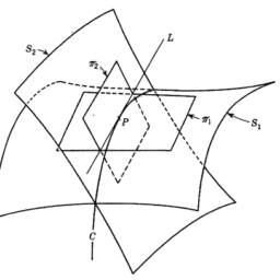
Consider a mass particle, which moves under the action of a force. Let the positive constant $m$ be the particle mass and $F=F(x, t)$ the force field. Here $x$ in $\mathbb{R}^d$ is the position variable ( $d=3$ in physical space but there is at this point no mathematical reason why $m$ cannot be an arbitrary positive integer) and $t>0$ the time. The force field is a $d$-dimensional vector field on $\mathbb{R}^d$, possibly time dependent. By $v \in \mathbb{R}^d$ we denote the velocity variable. Then the motion of the particle is characterized by the Newtonian phase space (i.e. $\mathbb{R}_x^d \times \mathbb{R}_v^d$ ) trajectories, which satisfy the system of ordinary differential equations (ODEs):
$$
\begin{gathered}
\dot{x}=v \
\dot{v}=\frac{1}{m} F(x, t) .
\end{gathered}
$$
Note that the first equation simply states that the particle’s velocity is the time derivative of its position and the second equation is just Newton’s ${ }^1$ celebrated second law, stating
$$
\text { force }=\text { mass } \cdot \text { acceleration } .
$$
If the field $F$ is sufficiently smooth, then by standard ODE theory we conclude that, given an initial state
$$
(x(t=0), v(t=0))=\left(x_0, v_0\right) \in \mathbb{R}^{2 d}
$$
there exists a locally defined, unique and smooth trajectory $\left(x\left(t ; x_0, v_0\right)\right.$, $\left.v\left(t ; x_0, v_0\right)\right)$. Thus, given the force and the initial position and velocity, the motion of the mass particle is – in the framework of classical Newtonian mechanics completely determined. However, in many applications, there are additional complications …
Assume at first that the intial state $\left(x_0, v_0\right)$ is not known a priorily, instead let $f_0=f_0(x, v)$ be a given probability distribution of the initial state, i.e. $f_0$ is non-negative, its integral over the whole phase space is 1 and, for any measurable subset $A$ of the phase space,
$$
\int_A f_0(x, v) d x d v=: P_0(A)
$$
is the probability of finding the particle at time $t=0$ in the set $A$. Then, instead of calculating the evolution of the phase space trajectories we can try to compute the location probability density $f=f(x, v, t)$, evolving out of $f_0$. For this we impose the condition that $f$ remains constant along the Newtonian trajectories:
$$
\frac{d}{d t} f\left(x\left(t ; x_0, v_0\right), v\left(t ; x_0, v_0\right), t\right)=0 .
$$
Carrying out the differentiation with respect to time, taking into account the Newtonian equations $(1.1,1.2)$ and renaming coordinates gives the so called Liouville equation:
$$
f_t+v \cdot \operatorname{grad}_x f+\frac{1}{m} F \cdot \operatorname{grad}_v f=0, \quad x \in \mathbb{R}^d, v \in \mathbb{R}^d ;, t>0,
$$
subject to the initial condition
$$
f(t=0)=f_0 .
$$

数学代写|偏微分方程代考Partial Differential Equations代写|The Navier-Stokes and Euler Equations Fluid and Gas Dynamics

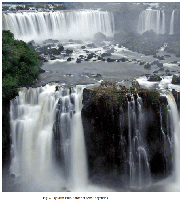
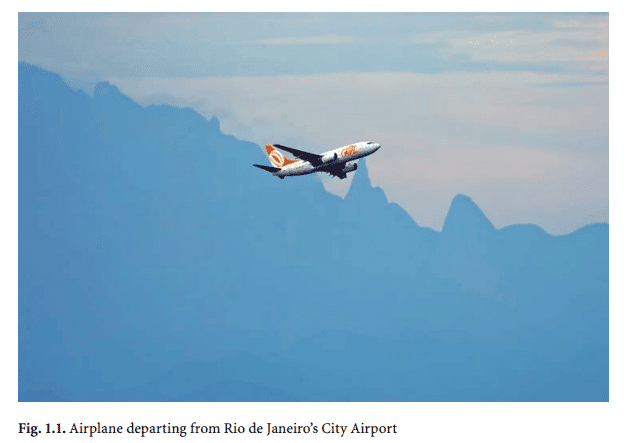
Fluid and gas dynamics have a decisive impact on our daily lives. There are the fine droplets of water which sprinkle down in our morning shower, the waves which we face swimming or surfing in the ocean, the river which adapts to the topography by forming a waterfall, the turbulent air currents which often disturb our transatlantic flight in a jet plane, the tsunami ${ }^1$ which can wreck an entire region of our world, the athmospheric flows creating tornados ${ }^2$ and hurricanes ${ }^3$, the live-giving flow of blood in our arteries and veins ${ }^4 \ldots$. All these flows have a great complexity from the geometrical, (bio)physical and (bio)mechanical viewpoints and their mathematical modeling is a highly challenging task.
Clearly, the dynamics of fluids and gases is governed by the interaction of their atoms/molecules, which theoretically can be modeled microscopically, i.e. by individual particle dynamics, relying on a grand Hamiltonian function depending on $3 N$ space coordinates and $3 N$ momentum coordinates, where $N$ is the number of particles in the fluid/gas. Note that the Newtonian ensemble trajectories live in $6 \mathrm{~N}$ dimensional phase space! For most practical purposes this is prohibitive and it is essential to carry out the thermodynamic BoltzmannGrad limit, which – under certain hypothesis on the particle interactions – gives the Boltzmann equation of gas dynamics (see Chapter 1 on kinetic equations) for the evolution of the effective mass density function in 6-dimensional phase space.
Under the assumption of a small particle mean free path (i.e. in the collision dominated regime) a further approximation is possible, leading to timedependent macroscopic equations in position space $\mathbb{R}^3$, referred to as NavierStokes and Euler systems. These systems of nonlinear partial differential equations are absolutely central in the modeling of fluid and gas flows.
For more (precise) information on this modeling hierarchy we refer to [3].
The Navier-Stokes system ${ }^5$ was written down in the 19th century. It is named after the French engineer and physicist Claude-Luis Navier ${ }^6$ and the Irish mathematician and physicist George Gabriel Stokes ${ }^7$.
Under the assumption of incompressibility of the fluid the Navier-Stokes equations, determining the fluid velocity $u$ and the fluid pressure $p$, read:
$$
\begin{aligned}
\frac{\partial u}{\partial t}+(u \cdot \operatorname{grad}) u+ & \operatorname{grad} p=v \Delta u+f \
\operatorname{div} u & =0
\end{aligned}
$$
Here $x$ denotes the space variable in $\mathbb{R}^2$ or $\mathbb{R}^3$ depending on whether 2 or 3 dimensional flows are to be modeled and $t>0$ is the time variable. The velocity field $u=u(x, t)$ (vector field on $\mathbb{R}^2$ or, resp., $\mathbb{R}^3$ ) is in $\mathbb{R}^2$ or $\mathbb{R}^3$, resp., and the pressure $p=p(x, t)$ is a scalar function. $f=f(x, t)$ is the (given) external force field (again two and, resp. three-dimensional) acting on the fluid and $v>0$ the kinematic viscosity parameter. The functions $u$ and $p$ are the solutions of the PDE system, the fluid density is assumed to be constant (say, 1) here as consistent with the incompressibility assumption. The nonlinear Navier-Stokes system has to be supplemented by an initial condition for the velocity field and by boundary conditions if spatially confined fluid flows are considered (or by decay conditions on whole space). A typical boundary condition is the so-called no-slip condition which reads
$$
u=0
$$
on the boundary of the fluid domain.
The constraint div $u=0$ enforces the incompressibility of the fluid and serves to determine the pressure $p$ from the evolution equation for the fluid velocity $u$.
If $v=0$ then the so called incompressible Euler ${ }^8$ equations, valid for very small viscosity flows (ideal fluids), are obtained. Note that the viscous NavierStokes equations form a parabolic system while the Euler equations (inviscid case) are hyperbolic. The Navier-Stokes and Euler equations are based on Newton’s celebrated second law: force equals mass times acceleration. They are consistent with the basic physical requirements of mass, momentum and energy conservation.
The incompressible Navier-Stokes and Euler equations allow an interesting simple interpretation, when they are written in terms of the fluid vorticity, defined by
$$
\omega:=\operatorname{curl} u
$$

偏微分方程代写

数学代写|偏微分方程代考Partial Differential Equations代写|Kinetic Equations: From Newton to Boltzmann

考虑一个质点，它在力的作用下运动。设正常数$m$为粒子质量$F=F(x, t)$为力场。这里$\mathbb{R}^d$中的$x$是位置变量($d=3$在物理空间中，但此时没有数学上的理由说明$m$不能是任意的正整数)，$t>0$是时间。力场是$\mathbb{R}^d$上的$d$维矢量场，可能与时间有关。我们用$v \in \mathbb{R}^d$表示速度变量。然后用牛顿相空间(即$\mathbb{R}_x^d \times \mathbb{R}_v^d$)轨迹来表征粒子的运动，该轨迹满足常微分方程(ode)系统:
$$
\begin{gathered}
\dot{x}=v \
\dot{v}=\frac{1}{m} F(x, t) .
\end{gathered}
$$
请注意，第一个方程简单地说明了粒子的速度是其位置的时间导数，第二个方程只是牛顿${ }^1$著名的第二定律，说明
$$
\text { force }=\text { mass } \cdot \text { acceleration } .
$$
如果场$F$足够光滑，那么根据标准ODE理论我们可以得出，给定初始状态
$$
(x(t=0), v(t=0))=\left(x_0, v_0\right) \in \mathbb{R}^{2 d}
$$
存在一个局部定义的、唯一的、光滑的轨迹$\left(x\left(t ; x_0, v_0\right)\right.$, $\left.v\left(t ; x_0, v_0\right)\right)$。因此，给定力和初始位置和速度，在经典牛顿力学的框架内，质量粒子的运动是完全确定的。然而，在许多应用中，还存在额外的复杂性……
首先假设初始状态$\left(x_0, v_0\right)$优先级未知，设$f_0=f_0(x, v)$为初始状态的给定概率分布，即$f_0$非负，其在整个相空间上的积分为1，对于相空间的任意可测量子集$A$，
$$
\int_A f_0(x, v) d x d v=: P_0(A)
$$
是在集合$A$中找到时间$t=0$的粒子的概率。然后，代替计算相空间轨迹的演化，我们可以尝试计算位置概率密度$f=f(x, v, t)$，从$f_0$演化而来。为此，我们施加$f$沿牛顿轨迹保持不变的条件:
$$
\frac{d}{d t} f\left(x\left(t ; x_0, v_0\right), v\left(t ; x_0, v_0\right), t\right)=0 .
$$
对时间进行微分，考虑牛顿方程$(1.1,1.2)$并重命名坐标，得到所谓的Liouville方程:
$$
f_t+v \cdot \operatorname{grad}_x f+\frac{1}{m} F \cdot \operatorname{grad}_v f=0, \quad x \in \mathbb{R}^d, v \in \mathbb{R}^d ;, t>0,
$$
以初始条件为准
$$
f(t=0)=f_0 .
$$

数学代写|偏微分方程代考Partial Differential Equations代写|The Navier-Stokes and Euler Equations Fluid and Gas Dynamics

流体和气体动力学对我们的日常生活有着决定性的影响。早晨淋浴时洒下的细小水滴，在海里游泳或冲浪时遇到的海浪，因地形变化而形成瀑布的河流，经常扰乱我们乘坐喷气式飞机跨大西洋飞行的湍流气流，能摧毁世界上整个地区的海啸${ }^1$，造成龙卷风${ }^2$和飓风${ }^3$的大气气流，血液在我们的动脉和静脉中流动${ }^4 \ldots$。从几何、(生物)物理和(生物)力学的角度来看，所有这些流都具有很大的复杂性，它们的数学建模是一项极具挑战性的任务。
显然，流体和气体的动力学是由它们的原子/分子的相互作用决定的，理论上可以在微观上建模，即通过单个粒子动力学，依赖于依赖于$3 N$空间坐标和$3 N$动量坐标的大哈密顿函数，其中$N$是流体/气体中的粒子数。注意，牛顿系综轨迹存在于$6 \mathrm{~N}$维相空间!对于大多数实际目的来说，这是禁止的，并且必须执行热力学玻尔兹曼格拉德极限，它在粒子相互作用的某些假设下给出了气体动力学的玻尔兹曼方程(见第1章动力学方程)，用于6维相空间中有效质量密度函数的演化。
在小粒子平均自由路径的假设下(即在碰撞主导状态下)，进一步的近似是可能的，导致位置空间$\mathbb{R}^3$中与时间相关的宏观方程，称为NavierStokes和Euler系统。这些非线性偏微分方程组在流体和气体流动的建模中是绝对重要的。
关于这个建模层次的更多(精确)信息，我们参考[3]。
纳维-斯托克斯系统${ }^5$是在19世纪写下来的。它是以法国工程师和物理学家克劳德·路易斯·纳维尔${ }^6$和爱尔兰数学家和物理学家乔治·加布里埃尔·斯托克斯${ }^7$的名字命名的。
在流体不可压缩的假设下，确定流体速度$u$和流体压力$p$的Navier-Stokes方程为:
$$
\begin{aligned}
\frac{\partial u}{\partial t}+(u \cdot \operatorname{grad}) u+ & \operatorname{grad} p=v \Delta u+f \
\operatorname{div} u & =0
\end{aligned}
$$
这里$x$表示$\mathbb{R}^2$或$\mathbb{R}^3$中的空间变量，这取决于要建模的是二维流还是三维流，$t>0$是时间变量。速度场$u=u(x, t)$ ($\mathbb{R}^2$或上的矢量场)($\mathbb{R}^3$)的网址是$\mathbb{R}^2$或$\mathbb{R}^3$。，压强$p=p(x, t)$是标量函数。$f=f(x, t)$是(给定的)外力场(同样是2和，参见。三维)作用于流体和$v>0$运动粘度参数。函数$u$和$p$是PDE系统的解，这里假设流体密度为常数(例如1)，与不可压缩假设相一致。非线性Navier-Stokes系统必须有速度场的初始条件和边界条件来补充，如果考虑空间受限的流体流动(或整个空间的衰减条件)。一个典型的边界条件是所谓的无滑移条件，它为
$$
u=0
$$
在流体域的边界上。
约束div $u=0$加强了流体的不可压缩性，并用于从流体速度$u$的演化方程确定压力$p$。
如果$v=0$，则获得了适用于非常小粘度流动(理想流体)的所谓不可压缩欧拉${ }^8$方程。注意，粘性NavierStokes方程形成抛物型方程组，而欧拉方程(无粘性情况)是双曲型方程组。纳维-斯托克斯方程和欧拉方程是基于牛顿著名的第二定律:力等于质量乘以加速度。它们符合质量、动量和能量守恒的基本物理要求。
不可压缩的纳维-斯托克斯方程和欧拉方程给出了一个有趣的简单解释，当它们用流体涡度来表示时，定义为
$$
\omega:=\operatorname{curl} u
$$

数学代写|偏微分方程代考Partial Differential Equations代写 请认准exambang™. exambang™为您的留学生涯保驾护航。

微观经济学代写

微观经济学是主流经济学的一个分支，研究个人和企业在做出有关稀缺资源分配的决策时的行为以及这些个人和企业之间的相互作用。my-assignmentexpert™ 为您的留学生涯保驾护航 在数学Mathematics作业代写方面已经树立了自己的口碑, 保证靠谱, 高质且原创的数学Mathematics代写服务。我们的专家在图论代写Graph Theory代写方面经验极为丰富，各种图论代写Graph Theory相关的作业也就用不着 说。

线性代数代写

线性代数是数学的一个分支，涉及线性方程，如：线性图，如：以及它们在向量空间和通过矩阵的表示。线性代数是几乎所有数学领域的核心。

博弈论代写

现代博弈论始于约翰-冯-诺伊曼（John von Neumann）提出的两人零和博弈中的混合策略均衡的观点及其证明。冯-诺依曼的原始证明使用了关于连续映射到紧凑凸集的布劳威尔定点定理，这成为博弈论和数学经济学的标准方法。在他的论文之后，1944年，他与奥斯卡-莫根斯特恩（Oskar Morgenstern）共同撰写了《游戏和经济行为理论》一书，该书考虑了几个参与者的合作游戏。这本书的第二版提供了预期效用的公理理论，使数理统计学家和经济学家能够处理不确定性下的决策。

微积分代写

微积分，最初被称为无穷小微积分或 “无穷小的微积分”，是对连续变化的数学研究，就像几何学是对形状的研究，而代数是对算术运算的概括研究一样。

它有两个主要分支，微分和积分；微分涉及瞬时变化率和曲线的斜率，而积分涉及数量的累积，以及曲线下或曲线之间的面积。这两个分支通过微积分的基本定理相互联系，它们利用了无限序列和无限级数收敛到一个明确定义的极限的基本概念 。

计量经济学代写

什么是计量经济学？
计量经济学是统计学和数学模型的定量应用，使用数据来发展理论或测试经济学中的现有假设，并根据历史数据预测未来趋势。它对现实世界的数据进行统计试验，然后将结果与被测试的理论进行比较和对比。

根据你是对测试现有理论感兴趣，还是对利用现有数据在这些观察的基础上提出新的假设感兴趣，计量经济学可以细分为两大类：理论和应用。那些经常从事这种实践的人通常被称为计量经济学家。

Matlab代写

MATLAB 是一种用于技术计算的高性能语言。它将计算、可视化和编程集成在一个易于使用的环境中，其中问题和解决方案以熟悉的数学符号表示。典型用途包括：数学和计算算法开发建模、仿真和原型制作数据分析、探索和可视化科学和工程图形应用程序开发，包括图形用户界面构建MATLAB 是一个交互式系统，其基本数据元素是一个不需要维度的数组。这使您可以解决许多技术计算问题，尤其是那些具有矩阵和向量公式的问题，而只需用 C 或 Fortran 等标量非交互式语言编写程序所需的时间的一小部分。MATLAB 名称代表矩阵实验室。MATLAB 最初的编写目的是提供对由 LINPACK 和 EISPACK 项目开发的矩阵软件的轻松访问，这两个项目共同代表了矩阵计算软件的最新技术。MATLAB 经过多年的发展，得到了许多用户的投入。在大学环境中，它是数学、工程和科学入门和高级课程的标准教学工具。在工业领域，MATLAB 是高效研究、开发和分析的首选工具。MATLAB 具有一系列称为工具箱的特定于应用程序的解决方案。对于大多数 MATLAB 用户来说非常重要，工具箱允许您学习和应用专业技术。工具箱是 MATLAB 函数（M 文件）的综合集合，可扩展 MATLAB 环境以解决特定类别的问题。可用工具箱的领域包括信号处理、控制系统、神经网络、模糊逻辑、小波、仿真等。