MY-ASSIGNMENTEXPERT™可以为您提供 soe.ucsc.edu STAT209 Generalized Linear Models广义线性模型的代写代考和辅导服务!
这是圣克鲁斯加利福尼亚大学 广义线性模型的代写成功案例。
STAT209课程简介
Theory, methods, and applications of generalized linear statistical models; review of linear models; binomial models for binary responses (including logistical regression and probit models); log-linear models for categorical data analysis; and Poisson models for count data. Case studies drawn from social, engineering, and life sciences.
Course description and background: This is a graduate-level course on the theory, methods and applications of Generalized Linear Models (GLMs). Emphasis will be placed on statistical modeling, building from standard normal linear models, extending to GLMs, and briefly covering more specialized topics. With regard to inference, prediction, and model assessment, we will study both likelihood and Bayesian methods. In particular, within the Bayesian modeling framework, we will discuss practically important hierarchical extensions of the standard GLM setting.
Prerequisites
Note that this is a course on methods for GLMs, rather than a course on using software for data analysis with GLMs. Students will be expected to be familiar with statistical software R, which will be used to illustrate the methods with data examples as part of the homework assignments (and exam). For data analysis problems involving Bayesian GLMs, you will be expected to write your own programs to fit Bayesian models using Markov chain Monte Carlo posterior simulation methods (R will suffice for this).
STAT209 Generalized Linear Models HELP(EXAM HELP, ONLINE TUTOR)
Shouki and Pause (1999) report data from a study of hormonal therapy for the treatment of cattle with cystic ovarian disease. One group received the hormone treatment of cattle with cystic ovarian disease and the other a placebo. The time recorded was the time to the complete disappearance of all cysts. An asterisk denotes a right-censored time. The data were
$\begin{aligned} \text { Treatment group: } & 7,12,15,16,18,22^* \ \text { Control group: } & 19,24,18^, 20^, 22^, 27^, 30^* .\end{aligned}$
(a) Estimate the hazard ratio for the treatment group using a proportional hazard model assuming that the survival time $T$ follows a Weibull distribution with scale parameter $\lambda$ and shape parameter $\alpha$. Provide an approximate $95 \%$ confidence interval for the hazard ratio of the treatment group to control group. Plot the hazard and survival functions for the two groups.
(b) Fit a Cox’s proportional hazards model to the data. Estimate the hazard ratio and an approximate $95 \%$ confidence interval for the hazard ratio. Note that when the number at risk for any group equals to zero, set it to be 0.001 . Compare the result using the Cox’s proportional hazard model model with the proportional hazard model in (a).
The following table reports the number of errors $y_i$ out of $t_i$ (in thousand) signals received from two transmitters. Let $g_i=0,1$ indicate the first and second transmitters respectively.
$\begin{array}{cccccccccccccc}y_i & 0 & 0 & 0 & 2 & 5 & 1 & 5 & 14 & 3 & 19 & 3 & 14 & 22 \ t_i & 25 & 37 & 41 & 42 & 94 & 16 & 63 & 126 & 5 & 31 & 7 & 24 & 36 \ g_i & 0 & 0 & 0 & 0 & 0 & 0 & 0 & 0 & 1 & 1 & 1 & 1 & 1\end{array}$
Conduct the following analyses.
(a) Fit the model
$$
Y_i \sim \mathcal{P}\left(\lambda_i t_i\right) \text { where } \lambda_i=\exp \left(\beta_0+\beta_1 g_i\right)
$$
to the data using a glm module in $\mathrm{R}$. Refit the model using negative binomial distribution. Compare the model fits.
(b) Suppose the information on the number of signal received $t_i$ is unavailable, refit the models in (a). Compare the model fits and state the cause(s) for the discrepancy of model fits in (a) and (b).
(c) Suppose the information on the number of signal received $t_i$ and the transmitter $b_i$ are both unavailable and the zero-inflated Poisson model with parameters $\lambda$ for the mean of Poisson distribution and $\pi$ for the proportion of zeros is fitted to the data.
(i) Prove the result for moment estimators
$$
\tilde{\lambda}=\frac{s^2-\bar{y}+\bar{y}^2}{\bar{y}} \text { and } \tilde{\pi}=\frac{s^2-\bar{y}}{s^2-\bar{y}+\bar{y}^2}
$$
where $\bar{y}$ is the sample mean and $s^2$ is the sample variance. Use the result to find the moment estimates, $\tilde{\lambda}$ and $\tilde{\pi}$.
(ii) Prove the result for maximum likelihood (ML) estimators
$$
\bar{y}\left(1-e^{-\hat{\lambda}}\right)=\hat{\lambda}\left(1-\frac{n_0}{n}\right) \text { and } \hat{\pi}=1-\frac{\bar{y}}{\hat{\lambda}}
$$
where $n_0$ is the number of zeros in the data, $\hat{\lambda}$ is the solution to the first equation and $\hat{\pi}$ depends on $\hat{\lambda}$. Use the $\mathrm{R}$ module uniroot to solve for the first equation to obtain $\hat{\lambda}$ and then calculate $\hat{\pi}$ using $\hat{\lambda}$.
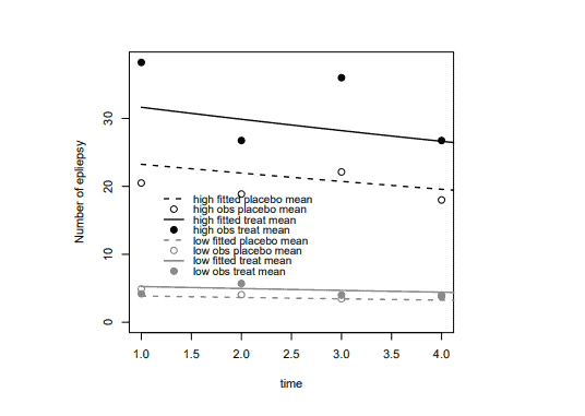
The epilepsy data were collected from a clinical trial of 59 epileptics by Leppik et al. (1985). In the randomized controlled trial, $m=59$ patients suffering from simple or complex partial seizures were assigned to either an antiepileptic drug progabide $\left(x_i=1\right)$ or a placebo $\left(x_i=0\right)$ with no intrinsic therapeutic value. The seizure counts were recorded at a two-week interval for an eight-week period $\left(n_i=4\right)$ with no dropout or missing cases.
Let $y_{i j}, i=1, \ldots, 59 ; j=1, \ldots, 4$ be the observed data. The covariates are time (1 to 4$)$, type (of treatment $x_i=0,1$ ), base and age. The data are stored in epilepsy.txt. The two covariates base and age are tested to be insignificant. Three mixture Poisson regression models, namely 1-group mixture (M1), 2-group mixture with group-specific intercept (M2) and 2-group mixture with group-specific intercept and time effect (M3), are considered. The mean functions for these 3 models are given below:
$$
\begin{array}{ll}
\text { M1: } & \mu_{i j}=\exp \left(\beta_0+\beta_1 \times j+\beta_2 x_i\right) \
\text { M2: } & \left{\begin{array}{l}
\mu_{i j 1}=\exp \left(\beta_{01}+\beta_1 \times j+\beta_2 x_i\right) \
\mu_{i j 2}=\exp \left(\beta_{02}+\beta_1 \times j+\beta_2 x_i\right)
\end{array}\right. \
\text { M3: } \quad\left{\begin{array}{l}
\mu_{i j 1}=\exp \left(\beta_{01}+\beta_{11} \times j+\beta_2 x_i\right) \
\mu_{i j 2}=\exp \left(\beta_{02}+\beta_{12} \times j+\beta_2 x_i\right)
\end{array}\right.
\end{array}
$$
$>$ dat=read.table (“Epilepsy.txt”, header $=\mathrm{T}$ )
$>$ pat=dat $[, 1]$; time=dat $[, 2]$; $\mathrm{y}=\operatorname{dat}[, 3]$; treatment=dat $[, 4]$; base=dat $[, 5]$; age=dat $[, 6]$
(a) Provide summary statistics for the seizure counts across time for all patients and for patients in treatment and placebo groups.
(b) Fit the three models using optim. Report parameter estimates, standard error and AIC.
(c) Choose the best model according to AIC. Report the group memberships, group sizes and observed and fitted means across time for the four groups of high-low by treatmentplacebo. Plot the observed and fitted means across time for these four groups. By comparing the observed mean and variance across time for the four groups, comment if other distribution will provide better model-fit.
Please attach your $\mathrm{R}$ commands.

MY-ASSIGNMENTEXPERT™可以为您提供 SOE.UCSC.EDU STAT209 GENERALIZED LINEAR MODELS广义线性模型的代写代考和辅导服务