MY-ASSIGNMENTEXPERT™可以为您提供sydney MATH3971 Convex Optimization凸优化课程的代写代考和辅导服务!
这是悉尼大学凸优化课程的代写成功案例。

MATH3971课程简介
The questions how to maximise your gain (or to minimise the cost) and how to determine the optimal strategy/policy are fundamental for an engineer, an economist, a doctor designing a cancer therapy, or a government planning some social policies. Many problems in mechanics, physics, neuroscience and biology can be formulated as optimistion problems. Therefore, optimisation theory is an indispensable tool for an applied mathematician. Optimisation theory has many diverse applications and requires a wide range of tools but there are only a few ideas underpinning all this diversity of methods and applications. This course will focus on two of them. We will learn how the concept of convexity and the concept of dynamic programming provide a unified approach to a large number of seemingly unrelated problems. By completing this unit you will learn how to formulate optimisation problems that arise in science, economics and engineering and to use the concepts of convexity and the dynamic programming principle to solve straight forward examples of such problems. You will also learn about important classes of optimisation problems arising in finance, economics, engineering and insurance.
Prerequisites
At the completion of this unit, you should be able to:
- LO1. analyse static optimisation problems with constraints
- LO2. formulate deterministic and stochastic dynamic optimisation problems, that arise in scientific and engineering applications, as mathematical problems
- LO3. understand the importance of convexity for optimisation problems, and use convexity to determine whether a solution to a given problem exists and is unique
- LO4. check if a certain controlled system is controllable, observable, stabilisable
- LO5. apply the Maximum Principle in order to solve real world control problems
- LO6. formulate the Hamilton-Jacobi-Bellman equation for solution of dynamic optimisation problems and solve them in special cases
- LO7. explain the derivations of key theoretical results and discuss the role of mathematical assumptions in these derivations
- LO8. use game theory to formulate optimisation problems with many competing players
- LO9. identify important solvable classes of optimisation problems arising in finance, economics, engineering and insurance and provide solutions.
MATH3971 Convex Optimization HELP(EXAM HELP, ONLINE TUTOR)
Approximation width. Let $f_0, \ldots, f_n: \mathbf{R} \rightarrow \mathbf{R}$ be given continuous functions. We consider the problem of approximating $f_0$ as a linear combination of $f_1, \ldots, f_n$. For $x \in \mathbf{R}^n$, we say that $f=x_1 f_1+\cdots+x_n f_n$ approximates $f_0$ with tolerance $\epsilon>0$ over the interval $[0, T]$ if $\left|f(t)-f_0(t)\right| \leq \epsilon$ for $0 \leq t \leq T$. Now we choose a fixed tolerance $\epsilon>0$ and define the approximation width as the largest $T$ such that $f$ approximates $f_0$ over the interval $[0, T]$ :
$$
W(x)=\sup \left{T|| x_1 f_1(t)+\cdots+x_n f_n(t)-f_0(t) \mid \leq \epsilon \text { for } 0 \leq t \leq T\right} .
$$
Show that $W$ is quasiconcave.
Solution. To show that $W$ is quasiconcave we show that the sets ${x \mid W(x) \geq \alpha}$ are convex for all $\alpha$. We have $W(x) \geq \alpha$ if and only if
$$
-\epsilon \leq x_1 f_1(t)+\cdots+x_n f_n(t)-f_0(t) \leq \epsilon
$$
for all $t \in[0, \alpha)$. Therefore the set ${x \mid W(x) \geq \alpha}$ is an intersection of infinitely many halfspaces (two for each $t$ ), hence a convex set.
Log-concavity of Gaussian cumulative distribution function. The cumulative distribution function of a Gaussian random variable,
$$
f(x)=\frac{1}{\sqrt{2 \pi}} \int_{-\infty}^x e^{-t^2 / 2} d t,
$$
is log-concave. This follows from the general result that the convolution of two logconcave functions is log-concave. In this problem we guide you through a simple self-contained proof that $f$ is log-concave. Recall that $f$ is log-concave if and only if $f^{\prime \prime}(x) f(x) \leq f^{\prime}(x)^2$ for all $x$.
(a) Verify that $f^{\prime \prime}(x) f(x) \leq f^{\prime}(x)^2$ for $x \geq 0$. That leaves us the hard part, which is to show the inequality for $x<0$.
(b) Verify that for any $t$ and $x$ we have $t^2 / 2 \geq-x^2 / 2+x t$.
(c) Using part (b) show that $e^{-t^2 / 2} \leq e^{x^2 / 2-x t}$. Conclude that
$$
\int_{-\infty}^x e^{-t^2 / 2} d t \leq e^{x^2 / 2} \int_{-\infty}^x e^{-x t} d t .
$$
(d) Use part (c) to verify that $f^{\prime \prime}(x) f(x) \leq f^{\prime}(x)^2$ for $x \leq 0$.
Solution. The derivatives of $f$ are
$$
f^{\prime}(x)=e^{-x^2 / 2} / \sqrt{2 \pi}, \quad f^{\prime \prime}(x)=-x e^{-x^2 / 2} / \sqrt{2 \pi} .
$$
(a) $f^{\prime \prime}(x) \leq 0$ for $x \geq 0$.
(b) Since $t^2 / 2$ is convex we have
$$
t^2 / 2 \geq x^2 / 2+x(t-x)=x t-x^2 / 2 .
$$
This is the general inequality
$$
g(t) \geq g(x)+g^{\prime}(x)(t-x),
$$
which holds for any differentiable convex function, applied to $g(t)=t^2 / 2$. Another (easier?) way to establish $t^2 / 2 \leq-x^2 / 2+x t$ is to note that
$$
t^2 / 2+x^2 / 2-x t=(1 / 2)(x-t)^2 \geq 0 .
$$
Now just move $x^2 / 2-x t$ to the other side.
(c) Take exponentials and integrate.
(d) This basic inequality reduces to
$$
-x e^{-x^2 / 2} \int_{-\infty}^x e^{-t^2 / 2} d t \leq e^{-x^2}
$$
i.e.,
$$
\int_{-\infty}^x e^{-t^2 / 2} d t \leq \frac{e^{-x^2 / 2}}{-x} .
$$
This follows from part (c) because
$$
\int_{-\infty}^x e^{-x t} d t=\frac{e^{-x^2}}{-x}
$$
Consider the optimization problem
$$
\begin{array}{ll}
\text { minimize } & f_0\left(x_1, x_2\right) \
\text { subject to } & 2 x_1+x_2 \geq 1 \
& x_1+3 x_2 \geq 1 \
& x_1 \geq 0, \quad x_2 \geq 0 .
\end{array}
$$
Make a sketch of the feasible set. For each of the following objective functions, give the optimal set and the optimal value.
(a) $f_0\left(x_1, x_2\right)=x_1+x_2$.
(b) $f_0\left(x_1, x_2\right)=-x_1-x_2$.
(c) $f_0\left(x_1, x_2\right)=x_1$.
(d) $f_0\left(x_1, x_2\right)=\max \left{x_1, x_2\right}$.
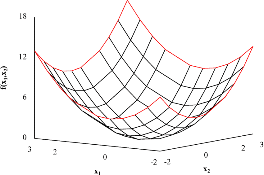
(e) $f_0\left(x_1, x_2\right)=x_1^2+9 x_2^2$.
Solution. The feasible set is shown in the figure.
(a) $x^{\star}=(2 / 5,1 / 5)$.
(b) Unbounded below.
(c) $X_{\text {opt }}=\left{\left(0, x_2\right) \mid x_2 \geq 1\right}$.
(d) $x^{\star}=(1 / 3,1 / 3)$.
(e) $x^{\star}=(1 / 2,1 / 6)$. This is optimal because it satisfies $2 x_1+x_2=7 / 6>1, x_1+3 x_2=$ 1 , and
$$
\nabla f_0\left(x^{\star}\right)=(1,3)
$$
is perpendicular to the line $x_1+3 x_2=1$.

MY-ASSIGNMENTEXPERT™可以为您提供SYDNEY MATH3971 CONVEX OPTIMIZATION凸优化课程的代写代考和辅导服务!