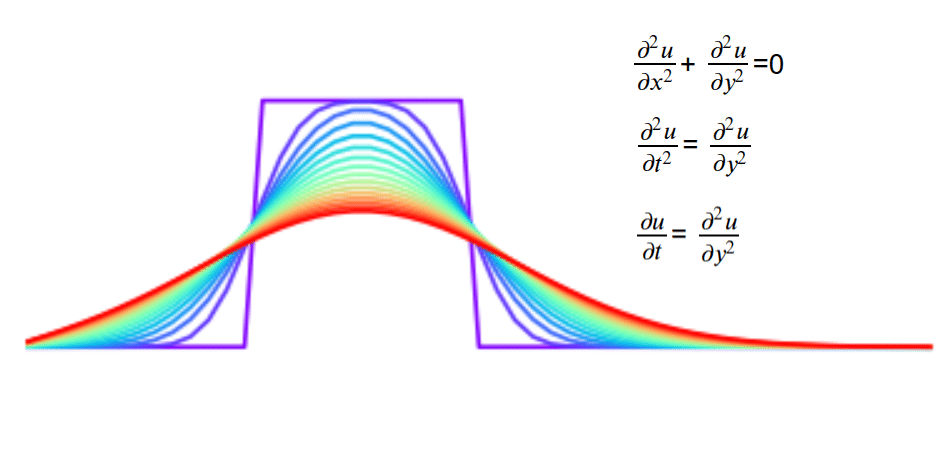
如果你也在 怎样代写偏微分方程Partial Differential Equations 这个学科遇到相关的难题,请随时右上角联系我们的24/7代写客服。偏微分方程Partial Differential Equations在数学中,偏微分方程(PDE)是一个方程,它规定了一个多变量函数的各种偏导数之间的关系。常微分方程构成了偏微分方程的一个子类,对应于单变量函数。截至2020年,随机偏微分方程和非局部方程是 “PDE “概念的特别广泛研究的延伸。更为经典的课题包括椭圆和抛物线偏微分方程、流体力学、玻尔兹曼方程和色散偏微分方程,目前仍有很多积极的研究。
偏微分方程Partial Differential Equations在以数学为导向的科学领域,如物理学和工程学中无处不在。例如,它们是现代科学对声音、热量、扩散、静电、电动力学、热力学、流体动力学、弹性、广义相对论和量子力学(薛定谔方程、保利方程等)的基础性认识。它们也产生于许多纯粹的数学考虑,如微分几何和变分计算;在其他值得注意的应用中,它们是几何拓扑学中证明庞加莱猜想的基本工具。部分由于这种来源的多样性,存在着广泛的不同类型的偏微分方程,并且已经开发了处理许多出现的个别方程的方法。因此,人们通常认为,偏微分方程没有 “一般理论”,专业知识在一定程度上被划分为几个基本不同的子领域。
同学们在留学期间,都对各式各样的作业考试很是头疼,如果你无从下手,不如考虑my-assignmentexpert™!
my-assignmentexpert™提供最专业的一站式服务:Essay代写,Dissertation代写,Assignment代写,Paper代写,Proposal代写,Proposal代写,Literature Review代写,Online Course,Exam代考等等。my-assignmentexpert™专注为留学生提供Essay代写服务,拥有各个专业的博硕教师团队帮您代写,免费修改及辅导,保证成果完成的效率和质量。同时有多家检测平台帐号,包括Turnitin高级账户,检测论文不会留痕,写好后检测修改,放心可靠,经得起任何考验!
数学代写|偏微分方程代考Partial Differential Equations代写|Statement and Proof of the Theorem
Consider the system of partial differential equations
$$
\frac{\partial u_i}{\partial x_n}=\sum_{k=1}^{n-1} \sum_{j=1}^N a_{i j}^k(\mathbf{p}) \frac{\partial u_j}{\partial x_k}+b_i(\mathbf{p}), \quad i=1, \ldots, N,
$$
where $\mathbf{p}$ stands for the vector $\left(x_1, \ldots, x_{n-1}, u_1, \ldots, u_N\right)$, with the initial conditions
$$
u_i=0 \quad \text { on } x_n=0, \quad i=1, \ldots, N .
$$
We shall establish the following local existence result.
Theorem 2.22. Let the functions $a_{i j}^k$ and $b_i$ be real analytic at the origin of $\mathbb{R}^{N+n-1}$. Then the system (2.65) with initial conditions (2.66) has a unique (among real analytic functions) system of solutions $u_i$ that is real analytic at the origin.
Proof. We begin by formally computing all derivatives of the $u_i$ at the origin. From (2.66) it follows that all tangential derivatives of all orders are zero. Hence the only nonzero first derivative is in the $x_n$ direction, and (2.65) leads to $\partial u_i / \partial x_n(\mathbf{0})=b_i(\mathbf{0})$. Next, we can differentiate (2.65) to obtain second derivatives of $u_i$. We find
$$
\frac{\partial^2 u_i}{\partial x_n \partial x_l}(\mathbf{0})=\sum_{k=1}^{n-1} \sum_{j=1}^N a_{i j}^k(\mathbf{0}) \frac{\partial^2 u_j}{\partial x_k \partial x_l}(\mathbf{0})+\sum_{j=1}^{N+n-1} \frac{\partial b_i}{\partial p_j}(\mathbf{0}) \frac{\partial p_j}{\partial x_l}(\mathbf{0}),
$$
which yields, for $l=1, \ldots, n-1$,
$$
\frac{\partial^2 u_i}{\partial x_n \partial x_l}=\frac{\partial b_i}{\partial p_l},
$$
and, for $l=n, i=1, \ldots, N$,
$$
\begin{aligned}
\frac{\partial^2 u_i}{\partial x_n^2} & =\sum_{k=1}^{n-1} \sum_{j=1}^N a_{i j}^k(\mathbf{0}) \frac{\partial^2 u_j}{\partial x_k \partial x_n}(\mathbf{0})+\sum_{j=1}^N \frac{\partial b_i}{\partial p_{n-1+j}}(\mathbf{0}) \frac{\partial u_j}{\partial x_n}(\mathbf{0}) \
& =\sum_{k=1}^{n-1} \sum_{j=1}^N a_{i j}^k(\mathbf{0}) \frac{\partial b_j}{\partial p_k}(\mathbf{0})+\sum_{j=1}^N \frac{\partial b_i}{\partial p_{n-1+j}}(\mathbf{0}) b_j(\mathbf{0}) .
\end{aligned}
$$
数学代写|偏微分方程代考Partial Differential Equations代写|Reduction of General Systems
We now consider a general system of partial differential equations, for which we shall prescribe initial data on a noncharacteristic surface. We shall demonstrate how such a problem can be reduced to the form given by (2.45), (2.46). First, we reduce the initial surface to a plane.
A surface is usually described in one of three ways:
- As a level set of a function: $\phi\left(x_1, \ldots, x_n\right)=\lambda$. Here it is assumed that $\nabla \phi \neq 0$.
- As a graph: $x_i=\psi\left(x_1, \ldots, x_{i-1}, x_{i+1}, \ldots, x_n\right)$.
- By a parametrization, $\mathbf{x}=\mathbf{F}(\mathbf{y})$, where $\mathbf{y} \in \mathbb{R}^{n-1}$. Here it is assumed that the matrix $\partial F_i / \partial y_j$ has maximal rank.
We say that a surface is of class $C^k, k \geq 1$ (analytic) if, respectively, the functions $\phi, \psi, \mathbf{F}$ are of class $C^k$ (analytic). The implicit function theorem implies that locally all three definitions are equivalent. After possible renumbering of coordinates, we may therefore assume that an analytic surface is given in the form $x_n=\psi\left(x_1, \ldots, x_{n-1}\right)$, where $\psi$ is analytic. We now set $y_i=x_i$ for $i \leq n-1$ and $y_n=x_n-\psi\left(x_1, \ldots, x_{n-1}\right)$. In the new coordinates the initial surface is $y_n=0$. Henceforth we shall therefore assume that the initial surface is the plane $x_n=0$.
In reducing the equations, we shall sometimes have to differentiate equations with respect to $x_n$. We note that after such a differentiation, the plane $x_n=0$ remains a noncharacteristic surface of the new system. Moreover, if the differentiated equation is satisfied everywhere and the original equation is satisfied at $x_n=0$, then the original equation is satisfied everywhere. That is, whenever we differentiate an equation with respect to $x_n$, we shall view the original equation as a constraint which has to be satisfied by the initial data for the new system.
We now note that any system of PDEs can be made quasilinear by differentiating one or more of the equations with respect to $x_n$. Hence we can restrict our attention to quasilinear systems. Consider a system of the form
$$
\sum_{j=1}^N \sum_{|\alpha|=s_i+t_j} a_{i j}^\alpha\left(\mathbf{p}_i\right) D^\alpha u_j+b_i\left(\mathbf{p}_i\right)=0, \quad i=1, \ldots, N,
$$
where $s_i$ and $t_j$ are the weights assigned to the equations and dependent variables, respectively (cf. the discussion in Example 2.10), and where the vector $\mathbf{p}_i$ consists of all the independent variables and all derivatives of the dependent variables $u_j$ of orders less than $s_i+t_j$. Since only the sums $s_i+t_j$ are relevant, we can assume that all the $s_i$ are non-positive and all the $t_j$ are non-negative. By differentiating the $i$ th equation $-s_i$ times with respect to $x_n$, we can then make $s_i$ for the new system equal to zero. After doing so, a natural set of initial conditions is obtained by prescribing $\partial^l u^j / \partial x_n^l$ for $l=0, \ldots, t_j-1$. These initial conditions must be subjected to constraints arising from any equations which have been differentiated with respect to $x_n$.
偏微分方程代写
数学代写|偏微分方程代考Partial Differential Equations代写|Statement and Proof of the Theorem
考虑一个偏微分方程组
$$
\frac{\partial u_i}{\partial x_n}=\sum_{k=1}^{n-1} \sum_{j=1}^N a_{i j}^k(\mathbf{p}) \frac{\partial u_j}{\partial x_k}+b_i(\mathbf{p}), \quad i=1, \ldots, N,
$$
其中$\mathbf{p}$表示初始条件下的向量$\left(x_1, \ldots, x_{n-1}, u_1, \ldots, u_N\right)$
$$
u_i=0 \quad \text { on } x_n=0, \quad i=1, \ldots, N .
$$
我们将建立如下的局部存在性结果。
定理2.22。设函数$a_{i j}^k$和$b_i$在$\mathbb{R}^{N+n-1}$的原点为实解析函数。那么具有初始条件(2.66)的系统(2.65)有一个唯一的(在实解析函数中)解系统$u_i$,它在原点是实解析的。
证明。我们从计算原点处$u_i$的所有导数开始。由式(2.66)可知,所有阶的切向导数均为零。因此,唯一的非零一阶导数在$x_n$方向上,并且(2.65)导致$\partial u_i / \partial x_n(\mathbf{0})=b_i(\mathbf{0})$。接下来,我们可以微分(2.65)得到$u_i$的二阶导数。我们发现
$$
\frac{\partial^2 u_i}{\partial x_n \partial x_l}(\mathbf{0})=\sum_{k=1}^{n-1} \sum_{j=1}^N a_{i j}^k(\mathbf{0}) \frac{\partial^2 u_j}{\partial x_k \partial x_l}(\mathbf{0})+\sum_{j=1}^{N+n-1} \frac{\partial b_i}{\partial p_j}(\mathbf{0}) \frac{\partial p_j}{\partial x_l}(\mathbf{0}),
$$
对于$l=1, \ldots, n-1$,
$$
\frac{\partial^2 u_i}{\partial x_n \partial x_l}=\frac{\partial b_i}{\partial p_l},
$$
对于$l=n, i=1, \ldots, N$,
$$
\begin{aligned}
\frac{\partial^2 u_i}{\partial x_n^2} & =\sum_{k=1}^{n-1} \sum_{j=1}^N a_{i j}^k(\mathbf{0}) \frac{\partial^2 u_j}{\partial x_k \partial x_n}(\mathbf{0})+\sum_{j=1}^N \frac{\partial b_i}{\partial p_{n-1+j}}(\mathbf{0}) \frac{\partial u_j}{\partial x_n}(\mathbf{0}) \
& =\sum_{k=1}^{n-1} \sum_{j=1}^N a_{i j}^k(\mathbf{0}) \frac{\partial b_j}{\partial p_k}(\mathbf{0})+\sum_{j=1}^N \frac{\partial b_i}{\partial p_{n-1+j}}(\mathbf{0}) b_j(\mathbf{0}) .
\end{aligned}
$$
数学代写|偏微分方程代考Partial Differential Equations代写|Reduction of General Systems
我们现在考虑一个一般的偏微分方程组,我们将在非特征表面上规定初始数据。我们将演示如何将这样的问题简化为式(2.45)、式(2.46)给出的形式。首先,我们将初始曲面简化为一个平面。
表面通常有三种描述方式:
作为一个函数的级别集:$\phi\left(x_1, \ldots, x_n\right)=\lambda$。这里假设$\nabla \phi \neq 0$。
作为图表:$x_i=\psi\left(x_1, \ldots, x_{i-1}, x_{i+1}, \ldots, x_n\right)$。
通过参数化,$\mathbf{x}=\mathbf{F}(\mathbf{y})$,其中$\mathbf{y} \in \mathbb{R}^{n-1}$。这里假设矩阵$\partial F_i / \partial y_j$具有最大秩。
如果函数$\phi, \psi, \mathbf{F}$分别属于$C^k$(解析)类,则我们说曲面属于$C^k, k \geq 1$(解析)类。隐函数定理表明三种定义在局部是等价的。在可能的坐标重新编号之后,我们可以假设一个解析曲面以$x_n=\psi\left(x_1, \ldots, x_{n-1}\right)$的形式给出,其中$\psi$是解析曲面。现在我们为$i \leq n-1$和$y_n=x_n-\psi\left(x_1, \ldots, x_{n-1}\right)$设置$y_i=x_i$。在新的坐标下,初始曲面是$y_n=0$。因此,我们假定初始曲面为平面$x_n=0$。
在简化方程时,我们有时必须对$x_n$微分方程。我们注意到,在这样的微分之后,平面$x_n=0$仍然是新系统的非特征面。而且,如果微分方程处处满足,原方程在$x_n=0$处处处满足,则原方程处处满足。也就是说,每当我们对$x_n$微分一个方程时,我们将把原方程看作一个约束,这个约束必须由新系统的初始数据来满足。
我们现在注意到,通过对$x_n$微分一个或多个方程,任何偏微分方程系统都可以成为拟线性的。因此,我们可以将注意力限制在拟线性系统上。考虑一个这样的系统
$$
\sum_{j=1}^N \sum_{|\alpha|=s_i+t_j} a_{i j}^\alpha\left(\mathbf{p}_i\right) D^\alpha u_j+b_i\left(\mathbf{p}_i\right)=0, \quad i=1, \ldots, N,
$$
其中$s_i$和$t_j$分别是分配给方程和因变量的权重(参见例2.10中的讨论),其中向量$\mathbf{p}_i$由所有自变量和所有阶数小于$s_i+t_j$的因变量$u_j$的导数组成。因为只有和$s_i+t_j$是相关的,我们可以假设所有的$s_i$都是非正的,所有的$t_j$都是非负的。通过对$i$微分方程$-s_i$乘以对$x_n$的微分,我们可以使新系统的$s_i$等于零。这样做之后,通过将$l=0, \ldots, t_j-1$指定为$\partial^l u^j / \partial x_n^l$得到一组自然的初始条件。这些初始条件必须服从于对$x_n$求导的任何方程所产生的约束。

数学代写|偏微分方程代考Partial Differential Equations代写 请认准exambang™. exambang™为您的留学生涯保驾护航。
微观经济学代写
微观经济学是主流经济学的一个分支,研究个人和企业在做出有关稀缺资源分配的决策时的行为以及这些个人和企业之间的相互作用。my-assignmentexpert™ 为您的留学生涯保驾护航 在数学Mathematics作业代写方面已经树立了自己的口碑, 保证靠谱, 高质且原创的数学Mathematics代写服务。我们的专家在图论代写Graph Theory代写方面经验极为丰富,各种图论代写Graph Theory相关的作业也就用不着 说。
线性代数代写
线性代数是数学的一个分支,涉及线性方程,如:线性图,如:以及它们在向量空间和通过矩阵的表示。线性代数是几乎所有数学领域的核心。
博弈论代写
现代博弈论始于约翰-冯-诺伊曼(John von Neumann)提出的两人零和博弈中的混合策略均衡的观点及其证明。冯-诺依曼的原始证明使用了关于连续映射到紧凑凸集的布劳威尔定点定理,这成为博弈论和数学经济学的标准方法。在他的论文之后,1944年,他与奥斯卡-莫根斯特恩(Oskar Morgenstern)共同撰写了《游戏和经济行为理论》一书,该书考虑了几个参与者的合作游戏。这本书的第二版提供了预期效用的公理理论,使数理统计学家和经济学家能够处理不确定性下的决策。
微积分代写
微积分,最初被称为无穷小微积分或 “无穷小的微积分”,是对连续变化的数学研究,就像几何学是对形状的研究,而代数是对算术运算的概括研究一样。
它有两个主要分支,微分和积分;微分涉及瞬时变化率和曲线的斜率,而积分涉及数量的累积,以及曲线下或曲线之间的面积。这两个分支通过微积分的基本定理相互联系,它们利用了无限序列和无限级数收敛到一个明确定义的极限的基本概念 。
计量经济学代写
什么是计量经济学?
计量经济学是统计学和数学模型的定量应用,使用数据来发展理论或测试经济学中的现有假设,并根据历史数据预测未来趋势。它对现实世界的数据进行统计试验,然后将结果与被测试的理论进行比较和对比。
根据你是对测试现有理论感兴趣,还是对利用现有数据在这些观察的基础上提出新的假设感兴趣,计量经济学可以细分为两大类:理论和应用。那些经常从事这种实践的人通常被称为计量经济学家。
Matlab代写
MATLAB 是一种用于技术计算的高性能语言。它将计算、可视化和编程集成在一个易于使用的环境中,其中问题和解决方案以熟悉的数学符号表示。典型用途包括:数学和计算算法开发建模、仿真和原型制作数据分析、探索和可视化科学和工程图形应用程序开发,包括图形用户界面构建MATLAB 是一个交互式系统,其基本数据元素是一个不需要维度的数组。这使您可以解决许多技术计算问题,尤其是那些具有矩阵和向量公式的问题,而只需用 C 或 Fortran 等标量非交互式语言编写程序所需的时间的一小部分。MATLAB 名称代表矩阵实验室。MATLAB 最初的编写目的是提供对由 LINPACK 和 EISPACK 项目开发的矩阵软件的轻松访问,这两个项目共同代表了矩阵计算软件的最新技术。MATLAB 经过多年的发展,得到了许多用户的投入。在大学环境中,它是数学、工程和科学入门和高级课程的标准教学工具。在工业领域,MATLAB 是高效研究、开发和分析的首选工具。MATLAB 具有一系列称为工具箱的特定于应用程序的解决方案。对于大多数 MATLAB 用户来说非常重要,工具箱允许您学习和应用专业技术。工具箱是 MATLAB 函数(M 文件)的综合集合,可扩展 MATLAB 环境以解决特定类别的问题。可用工具箱的领域包括信号处理、控制系统、神经网络、模糊逻辑、小波、仿真等。