如果你也在 怎样代写流形学习Manifold learning 这个学科遇到相关的难题,请随时右上角联系我们的24/7代写客服。流形学习Manifold learning是一种用于机器学习的降维技术,旨在保留高维数据的底层结构,同时在低维环境中表示它。
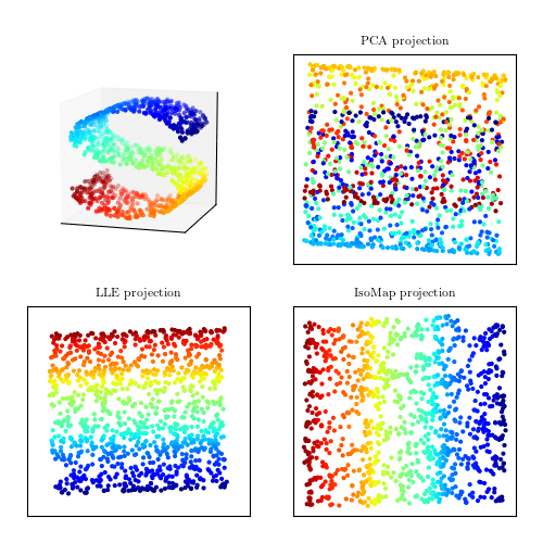
流形学习Manifold learningPCA识别数据中的三个主要成分。投影到前两个PCA分量导致沿歧管混合的颜色。流形学习(LLE和IsoMap)在投影数据时保留了局部结构,防止了颜色的混合。
流形学习Manifold learning代写,免费提交作业要求, 满意后付款,成绩80\%以下全额退款,安全省心无顾虑。专业硕 博写手团队,所有订单可靠准时,保证 100% 原创。 最高质量的流形学习Manifold learning作业代写,服务覆盖北美、欧洲、澳洲等 国家。 在代写价格方面,考虑到同学们的经济条件,在保障代写质量的前提下,我们为客户提供最合理的价格。 由于作业种类很多,同时其中的大部分作业在字数上都没有具体要求,因此流形学习Manifold learning作业代写的价格不固定。通常在专家查看完作业要求之后会给出报价。作业难度和截止日期对价格也有很大的影响。
同学们在留学期间,都对各式各样的作业考试很是头疼,如果你无从下手,不如考虑my-assignmentexpert™!
my-assignmentexpert™提供最专业的一站式服务:Essay代写,Dissertation代写,Assignment代写,Paper代写,Proposal代写,Proposal代写,Literature Review代写,Online Course,Exam代考等等。my-assignmentexpert™专注为留学生提供Essay代写服务,拥有各个专业的博硕教师团队帮您代写,免费修改及辅导,保证成果完成的效率和质量。同时有多家检测平台帐号,包括Turnitin高级账户,检测论文不会留痕,写好后检测修改,放心可靠,经得起任何考验!
计算机代写|流形学习代写Manifold learning代考|Multidimensional Scaling
Multidimensional scaling (MDS) is a family of algorithms each member of which seeks to identify an underlying manifold consistent with a given set of data. A useful motivation for MDS can be viewed in the following way. Imagine a map of a particular geographical region, which includes several cities and towns. Such a map is usually accompanied by a two-way table of distances between selected pairs of those towns and cities. The number in each cell of that table gives the degree of “closeness” (or proximity) of the row city to the column city that identifies that cell. The general problem of MDS reverses that relationship between the map and table of proximities. With MDS, one is given only the table of proximities, and the problem is to reconstruct the map as closely as possible. There is one more wrinkle: the number of dimensions of the map is unknown, and so we have to determine the dimensionality of the underlying (linear) manifold that is consistent with the given table of proximities.
Proximity Matrices
Proximities do not have to be distances, but can be a more complicated concept. We can talk about the proximity of any two entities to each other, where by “entity” we might mean an object, a brand-name product, a nation, a stimulus, and so on. The proximity of a pair of such entities could be a measure of association (e.g., the absolute value of a correlation coefficient), a confusion frequency (i.e., to what extent one entity is confused with another in an identification exercise), or some other measure of how alike (or how different) one perceives the entities to be. A proximity can be a continuous measure of how physically close one entity is to another or it could be a subjective judgment recorded on an ordinal scale, but where the scale is sufficiently well-calibrated as to be considered continuous. In other scenarios, especially in studies of perception, a proximity will not be quantitative, but will be a subjective rating of “similarity” (how close a pair of entities are to each other) or “dissimilarity” (how unalike are the pair of entities). The only thing that really matters in MDS is that there should be a monotonic relationship (either increasing or decreasing) between the “closeness” of two entities and the corresponding similarity or dissimilarity value.
计算机代写|流形学习代写Manifold learning代考|Classical Scaling
Although there are several different versions of MDS, we describe here only the classical scaling method. Other methods are described in Izenman (2008, Chapter 13).
So, suppose we are given $n$ points $\mathbf{X}1, \ldots, \mathbf{X}_n \in \Re^r$ from which we compute an $(n \times n)$ matrix $\boldsymbol{\Delta}=\left(\delta{i j}\right)$ of dissimilarities, where
$$
\delta_{i j}=\left|\mathbf{X}i-\mathbf{X}_j\right|=\left{\sum{k=1}^r\left(X_{i k}-X_{j k}\right)^2\right}^{1 / 2}
$$
is the dissimilarity between $\mathbf{X}i=\left(X{i 1}, \cdots, X_{i r}\right)^\tau$ and $\mathbf{X}j=\left(X{j 1}, \cdots, X_{j r}\right)^\tau, i, j=$ $1,2, \ldots, n$; these dissimilarities are the Euclidean distances between all $m=n(n-1) / 2$ pairs of points in that space. Squaring both sides of (1.23) and expanding the right-hand side yields
$$
\delta_{i j}^2=\left|\mathbf{X}i\right|^2+\left|\mathbf{X}_j\right|^2-2 \mathbf{X}_i^\tau \mathbf{X}_j $$ Note that $\delta{i 0}^2=\left|\mathbf{X}i\right|^2$ is the squared distance from the point $\mathbf{X}_i$ to the origin. Let $$ b{i j}=\mathbf{X}i^\tau \mathbf{X}_j=-\frac{1}{2}\left(\delta{i j}^2-\delta_{i 0}^2-\delta_{j 0}^2\right)
$$
Summing (1.24) over $i$ and over $j$ gives the following identities:
$$
\begin{aligned}
n^{-1} \sum_i \delta_{i j}^2 & =n^{-1} \sum_i \delta_{i 0}^2+\delta_{j 0}^2 \
n^{-1} \sum_j \delta_{i j}^2 & =\delta_{i 0}^2+n^{-1} \sum_j \delta_{j 0}^2 \
n^{-2} \sum_i \sum_j \delta_{i j}^2 & =2 n^{-1} \sum_i \delta_{i 0}^2 .
\end{aligned}
$$
Let $a_{i j}=-\frac{1}{2} \delta_{i j}^2$. Using the usual “dot” notation, we define $a_i .=n^{-1} \sum_j a_{i j}, a_{. j}=$ $n^{-1} \sum_i a_{i j}$, and $a . .=n^{-2} \sum_i \sum_j a_{i j}$. Substituting (1.26)-(1.28) into (1.25) and then simplifying, we get
$$
b_{i j}=a_{i j}-a_{i \cdot}-a_{. j}+a_{\ldots}
$$

流形学习代写
计算机代写|流形学习代写Manifold learning代考|Multidimensional Scaling
我们将在本章中描述的所有流形学习算法都假设有有限个数据点$\left{\mathbf{y}i\right}$是从光滑的$t$维流形$\mathcal{M}$随机抽取的,其度量由测地线距离$d^{\mathcal{M}}$给出。这些数据点(线性或非线性)通过平滑映射$\psi$嵌入到高维输入空间$\mathcal{X}=\Re^r$中,其中$t \ll r$与欧几里得度量$|\cdot|{\mathcal{X}}$。这种嵌入会产生输入数据点$\left{\mathbf{x}_i\right}$。换句话说,嵌入映射是$\psi: \mathcal{M} \rightarrow \mathcal{X}$,流形上的一个点$\mathbf{y}_i \in \mathcal{M}$可以表示为$\mathbf{y}=\phi(\mathbf{x}), \mathbf{x} \in \mathcal{X}$,其中$\phi=\psi^{-1}$。
目标是恢复$\mathcal{M}$并找到地图$\psi$的显式表示(并恢复${\mathbf{y}}$),给定$\mathcal{X}$中的输入数据点$\left{\mathbf{x}_i\right}$,或者这些点所有对之间的距离的接近矩阵。当我们应用这些算法时,我们获得了提供流形数据$\left{\mathbf{y}_i\right} \subset \Re^t$重建的估计$\left{\widehat{\mathbf{y}}_i\right} \subset \Re^{t^{\prime}}$,对于一些$t^{\prime}$。显然,如果$t^{\prime}=t$,我们已经成功了。通常,我们期望$t^{\prime}>3$,因此结果对于可视化目的是不切实际的。为了克服这个困难,在仍然提供低维表示的同时,我们只取重建坐标向量的前两个或三个点,并将它们绘制在二维或三维空间中。
计算机代写|流形学习代写Manifold learning代考|Classical Scaling
虽然MDS有几个不同的版本,但我们在这里只描述经典的缩放方法。Izenman(2008,第13章)描述了其他方法。
因此,假设我们给定$n$点$\mathbf{X}1, \ldots, \mathbf{X}n \in \Re^r$,从中我们计算不相似度的$(n \times n)$矩阵$\boldsymbol{\Delta}=\left(\delta{i j}\right)$,其中 $$ \delta{i j}=\left|\mathbf{X}i-\mathbf{X}j\right|=\left{\sum{k=1}^r\left(X{i k}-X_{j k}\right)^2\right}^{1 / 2}
$$
是$\mathbf{X}i=\left(X{i 1}, \cdots, X_{i r}\right)^\tau$和$\mathbf{X}j=\left(X{j 1}, \cdots, X_{j r}\right)^\tau, i, j=$$1,2, \ldots, n$的不同之处;这些不相似度是该空间中所有$m=n(n-1) / 2$点对之间的欧氏距离。(1.23)的两边平方,然后展开右边就得到
$$
\delta_{i j}^2=\left|\mathbf{X}i\right|^2+\left|\mathbf{X}j\right|^2-2 \mathbf{X}_i^\tau \mathbf{X}_j $$注意$\delta{i 0}^2=\left|\mathbf{X}i\right|^2$是从点$\mathbf{X}_i$到原点的距离的平方。让 $$ b{i j}=\mathbf{X}i^\tau \mathbf{X}_j=-\frac{1}{2}\left(\delta{i j}^2-\delta{i 0}^2-\delta_{j 0}^2\right)
$$
对$i$和$j$求和(1.24)得到以下等式:
$$
\begin{aligned}
n^{-1} \sum_i \delta_{i j}^2 & =n^{-1} \sum_i \delta_{i 0}^2+\delta_{j 0}^2 \
n^{-1} \sum_j \delta_{i j}^2 & =\delta_{i 0}^2+n^{-1} \sum_j \delta_{j 0}^2 \
n^{-2} \sum_i \sum_j \delta_{i j}^2 & =2 n^{-1} \sum_i \delta_{i 0}^2 .
\end{aligned}
$$
让$a_{i j}=-\frac{1}{2} \delta_{i j}^2$。使用通常的“点”表示法,我们定义$a_i .=n^{-1} \sum_j a_{i j}, a_{. j}=$$n^{-1} \sum_i a_{i j}$和$a . .=n^{-2} \sum_i \sum_j a_{i j}$。将(1.26)-(1.28)代入(1.25)化简,得到
$$
b_{i j}=a_{i j}-a_{i \cdot}-a_{. j}+a_{\ldots}
$$

计算机代写|流形学习代写Manifold learning代考 请认准UprivateTA™. UprivateTA™为您的留学生涯保驾护航。
微观经济学代写
微观经济学是主流经济学的一个分支,研究个人和企业在做出有关稀缺资源分配的决策时的行为以及这些个人和企业之间的相互作用。my-assignmentexpert™ 为您的留学生涯保驾护航 在数学Mathematics作业代写方面已经树立了自己的口碑, 保证靠谱, 高质且原创的数学Mathematics代写服务。我们的专家在图论代写Graph Theory代写方面经验极为丰富,各种图论代写Graph Theory相关的作业也就用不着 说。
线性代数代写
线性代数是数学的一个分支,涉及线性方程,如:线性图,如:以及它们在向量空间和通过矩阵的表示。线性代数是几乎所有数学领域的核心。
博弈论代写
现代博弈论始于约翰-冯-诺伊曼(John von Neumann)提出的两人零和博弈中的混合策略均衡的观点及其证明。冯-诺依曼的原始证明使用了关于连续映射到紧凑凸集的布劳威尔定点定理,这成为博弈论和数学经济学的标准方法。在他的论文之后,1944年,他与奥斯卡-莫根斯特恩(Oskar Morgenstern)共同撰写了《游戏和经济行为理论》一书,该书考虑了几个参与者的合作游戏。这本书的第二版提供了预期效用的公理理论,使数理统计学家和经济学家能够处理不确定性下的决策。
微积分代写
微积分,最初被称为无穷小微积分或 “无穷小的微积分”,是对连续变化的数学研究,就像几何学是对形状的研究,而代数是对算术运算的概括研究一样。
它有两个主要分支,微分和积分;微分涉及瞬时变化率和曲线的斜率,而积分涉及数量的累积,以及曲线下或曲线之间的面积。这两个分支通过微积分的基本定理相互联系,它们利用了无限序列和无限级数收敛到一个明确定义的极限的基本概念 。
计量经济学代写
什么是计量经济学?
计量经济学是统计学和数学模型的定量应用,使用数据来发展理论或测试经济学中的现有假设,并根据历史数据预测未来趋势。它对现实世界的数据进行统计试验,然后将结果与被测试的理论进行比较和对比。
根据你是对测试现有理论感兴趣,还是对利用现有数据在这些观察的基础上提出新的假设感兴趣,计量经济学可以细分为两大类:理论和应用。那些经常从事这种实践的人通常被称为计量经济学家。
Matlab代写
MATLAB 是一种用于技术计算的高性能语言。它将计算、可视化和编程集成在一个易于使用的环境中,其中问题和解决方案以熟悉的数学符号表示。典型用途包括:数学和计算算法开发建模、仿真和原型制作数据分析、探索和可视化科学和工程图形应用程序开发,包括图形用户界面构建MATLAB 是一个交互式系统,其基本数据元素是一个不需要维度的数组。这使您可以解决许多技术计算问题,尤其是那些具有矩阵和向量公式的问题,而只需用 C 或 Fortran 等标量非交互式语言编写程序所需的时间的一小部分。MATLAB 名称代表矩阵实验室。MATLAB 最初的编写目的是提供对由 LINPACK 和 EISPACK 项目开发的矩阵软件的轻松访问,这两个项目共同代表了矩阵计算软件的最新技术。MATLAB 经过多年的发展,得到了许多用户的投入。在大学环境中,它是数学、工程和科学入门和高级课程的标准教学工具。在工业领域,MATLAB 是高效研究、开发和分析的首选工具。MATLAB 具有一系列称为工具箱的特定于应用程序的解决方案。对于大多数 MATLAB 用户来说非常重要,工具箱允许您学习和应用专业技术。工具箱是 MATLAB 函数(M 文件)的综合集合,可扩展 MATLAB 环境以解决特定类别的问题。可用工具箱的领域包括信号处理、控制系统、神经网络、模糊逻辑、小波、仿真等。