MATH0066 (Nonlinear Systems)
Year:
Code:
Level:
Value:
Term:
Structure:
2020–2021
MATH0066
Masters
15 UCL credits (= 7.5 ECTS credits)
1
Online
Assessment: 100% examination. Weekly Homework Problem Sheets for practice
(marked and returned to provide feedback).
Lecturer: Professor SR Bishop
Course Description and Objectives
This module gives an overview of the main aspects of nonlinear systems that arise in continuous and discrete dynamical systems and aims to build the required skills to understand and
visualise various dynamical outcomes. It will provide basic definitions and indicate theoretical
background. Physical applications will be considered with an emphasis placed on combining
analytical treatments with an understanding of their practical implications in a modelling setting.
Recommended Texts
(i) S.H.Strogatz, Nonlinear Dynamics and Chaos, Perseus Books, 1994.
(ii) J.M.T.Thompson & H.B. Stewart, Nonlinear Dynamics and Chaos, Wiley 2003.
(iii) E.Ott, Chaos in Dynamical Systems, CUP, 1993.
(iv) D.K.Arrowsmith & C.M.Place, Dynamical Systems, Chapman Hall 1990.
(v) J. Guckenheimer and P. Holmes, Nonlinear Oscillations, Dynamical Systems and Bifurcations of Vector Fields, Springer 1983.
(vi) P.Drazin Nonlinear Systems, Cambridge University Press, 1992.
(vii) P.Drazin and R.S.Johnson, Solitons, Cambridge University Press, 1989.
(viii) L.D.Landau & E.M.Lifshitz, A Course of Theoretical Physics, Vol. 1 Mechanics, Pergamon
1960.
(ix) E.Infeld & G.Rowlands, Nonlinear Waves, Solitons and Chaos, CUP, 2000.
(x) L.N.Virgin, Introduction to Experimental Nonlinear Dynamics, CUP, 2000.
Detailed Syllabus
Introduction: Review of dynamics and modelling concepts. Deterministic versus probabilistic
models. The role of nonlinearity and damping/dissipation. Introduction to complex systems
and agent based modelling.
Continuous Dynamical Systems: Flows governed by ODEs. Transients and steady states –
equilibrium, periodic and chaotic solutions. Local and global stability. Liouville’s theorem.
Conservative and dissipative mechanical systems. Periodic solutions and Poincare-Bendixson
theorem. Bifurcation theory for 1- and 2-dimensional systems including structural stability
of bifurcations. Comparison of conservative systems and dissipative systems. Chaos and the
butterfly effect. Potential well dynamics for nonlinear oscillators. Numerical considerations
including basins of attraction, the role of unstable saddles, homoclinic/heteroclinic trajectories
and Lyapunov exponents. Link to maps via Poincar´e sections.
Discrete Dynamical Systems: Iterated maps as dynamical systems in discrete time. The logistic
map as main example. Fixed points, cycles and their stability. Period doubling and other
bifurcations of maps. Elementary properties of maps in two dimensions. Lyapunov exponents
for maps.
Spatial Temporal Dynamics:
Flows governed by PDEs. Linear waves, dispersion relations,
dissipation leading to stable waves. Travelling wave solutions of non-linear partial differential
equations, for example the Korteweg-de Vries. Solitons and link with homoclinic orbits of
potential well systems.
October 2020 MATH0066
If we imagine following a path of a chosen steady state solution to a nonlinear system then a bifurcation occurs when a parameter is slowly varied and there is a qualitative change in the system dynamics. In other words, subtle changes to a parameter result in vastly different long-term behaviour. A practical example might result in, for instance, a disease dying out or an epidemic taking hold in a community. Although this is not written in the usual mathematical jargon of $\varepsilon$ and $\delta$, in some sense, this is the definition of a bifurcation. Generally, a bifurcation means that we will see a change in the
– Stability of a solution
– Type of solution (e.g. an equilibrium changes to a periodic solution, but not when an equilibrium changes from being a node to focus, or vice versa) Number of solutions. Sometimes at a bifurcation we go from one solution to two solutions hence the prefix bi-, but instabilities are now also called bifurcations, as are phase transitions. The term bifurcate can thus be thought of as referring to the two types of behaviour; one before and one after the bifurcation. When we talk about local bifurcations, the term local means that we are considering the dynamics close to the equilibrium. In particular, it means that we are monitoring an equilibrium solution as we change a parameter and investigating changes to the eigenvalues that determine its stability. For flows, if $\lambda=\alpha+i \beta$ is the eigenvalue of the Jacobian matrix evaluated at the equilibrium point, then a bifurcation occurs when $\alpha=\operatorname{Re}(\lambda)=0$. If $\operatorname{Re}(\lambda)<0$ then the equilibrium is asymptotically stable, as visualised in Figure $2.29 .$ So, we could in fact define a local bifurcation of an equilibrium as taking place when $\operatorname{Re}(\lambda)=0$, where $\lambda$ is the eigenvalues of the Jacobian matrix evaluated at the equilibrium point.
Illustrative examples:
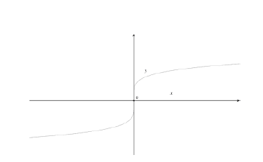
1) As seen in Nayfeh and Balachandran, consider the system $\dot{x}=\mu-x^{5}$. There is only one equilibrium state when $x=\mu^{1 / 5}$.
We see that the Jacobian is zero when evaluated at $x=\mu=0$ implying that the origin is indeed non-hyperbolic. However, no qualitative changes take place in the type of solution nor the number of solutions as we pass through $\mu=0$ and therefore no bifurcation takes place. That is to say, it is a good idea to set up an algorithm to find when $\operatorname{Re}(\lambda)=0$ since this will identify potential bifurcations, but in order to confirm that a bifurcation has taken place then we need to do more work.
For the moment we focus on the study of local bifurcations of equilibrium solutions but later we will also consider changes to periodic solutions. Both are equivalent to investigating the loss of hyperbolic behaviour.
The term generic is often used in this context and means typically under the variation of a single parameter with no symmetries or special constraints.
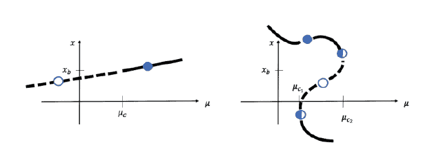
A bifurcation diagram is a plot of any representative value of the steady state (in the first instance in this section we restrict ourselves to the case when the solution is an equilibrium) as a single parameter, $\mu$, is varied. So we could plot $(\mu, x),(\mu, y)$ or $\left(\mu, x_{P}\right)$, where $x_{P}$ is the Poincaré point of the steady state. In driven systems, we have already seen the frequency of the driving force, $\omega$, can be used as a parameter (typically when considering periodic solutions) but for general descriptions we usually use the letter $\mu$ as the parameter. Later we can consider what happens to periodic solutions as a parameter is varied but for now we restrict our attention to equilibrium solutions. We plot the path of asymptotically stable equilibrium solutions with solid lines and unstable solutions with dashed lines. Two different scenarios are envisaged in following Figure,

space
To show that a certain parameter value leads to bifurcation point we can analytically show that the corresponding eigenvalue is such that $\alpha=\operatorname{Re}(\lambda)=0$, but to illustrate the dynamical change caused by the bifurcation we usually illustrate the behaviour by drawing, for instance, phase portraits, before, and then after the bifurcation. That is, we do not plot the diagram actually at the critical value since the dynamics here take a very long time to settle down (even for fixed levels of damping).
Our aim here is to try and classify the generic bifurcations that we see which are common to many different systems. In this way, when we describe the behaviour we will have a common understanding of the system response. However, in some cases solutions just appear, due to the nature of the equations or constraints on the parameters.

动力系统代写,数学代写dynamic system请认准UprivateTA™. UprivateTA™为您的留学生涯保驾护航。
偏微分方程代写
PDE代写
线性代数代写
Partial Differential Equations代写可以参考一份偏微分方程midterm答案解析


