MY-ASSIGNMENTEXPERT™可以为您提供 montana.edu EC1B1 Macroeconomics宏观经济学的代写代考和辅导服务!
这是伦敦政经学院宏观经济学课程的代写成功案例。
EC1B1课程简介
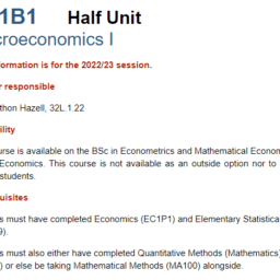
Teacher responsible
Dr Jonathon Hazell, 32L.1.22
Availability
This course is available on the BSc in Econometrics and Mathematical Economics and BSc in Economics. This course is not available as an outside option nor to General Course students.
Pre-requisites
Students must have completed Economics (EC1P1) and Elementary Statistical Theory I (ST109).
Students must also either have completed Quantitative Methods (Mathematics) (MA107) or else be taking Mathematical Methods (MA100) alongside.
Prerequisites
This course builds on the knowledge learned in EC1P1. You will learn why economic activity fluctuates over time (business cycles). We will discuss how government policy can affect short-term outcomes, such as unemployment, GDP and inflation. Other topics will include inequality and financial crises. We will apply the tools developed in the course to recent events, as well as historical events such as the Great Depression. An important aspect of the course is a coding exercise with data. This will help you acquire a deeper understanding of the material.
EC1B1, in combination with EC1A1, contributes towards certificate level exemptions from professional Chartered Institute of Management Accountants (CIMA) examinations.
This course, combined with EC1A1, contributes to the CB2 Exemption of the Institute and Faculty of Actuaries (IFoA).
EC1B1 Macroeconomics(EXAM HELP, ONLINE TUTOR)
Assume that population is equal to 1 . Consider the following IS-LM curve.
$$
\begin{gathered}
y=c(y-\tau)+\iota(\rho)+g \
\frac{m^s}{P}=k(\rho) y
\end{gathered}
$$
where price level $P$, tax revenue $\tau$, government expenditure $g$ and money supply $m^s$ are given. Two equations determine GDP, $y$ and the interest rate $\rho$. Suppose that
$$
\begin{aligned}
c(y-\tau) & =c_0+c_1 \times(y-\tau) \
k(\rho) & =\frac{k}{\rho} \
\iota(\rho) & =-a \rho
\end{aligned}
$$
where $c_0, c_1, k$, and $a$ are parameters.
What is the effect of an increase in tax revenue, $\tau$, on GDP and the interest rate? Explain economic logic behind your answer.
Answer We analyze the effect of an increase in tax revenue, $\tau$, on GDP and the interest rate. Note that IS curve depends on $\tau$ but LM curve does not depend on $\tau$. When tax revenue increases, IS curve shifts down (See Figure 2). Both GDP and the interest rate decrease. The economic logic for this result is as follows. First, IS curve implies that an increase in $\tau$ directly decreases demand and GDP (see (IS)):
$$
\tau \uparrow \Rightarrow y \downarrow
$$
Second, the decrease in GDP reduces the demand for money $\left(m^d\right)$. When the price level and money supply are constant, this actually decreases the interest rate in the money market (see (LM)):
$$
\tau \uparrow \Rightarrow y \downarrow \Rightarrow m^d \downarrow \Rightarrow \rho \downarrow
$$
Since investment $i=\iota(\rho)=-a \rho$, a decrease in $\rho$ leads to an increase in the investment $i$ :
$$
\tau \uparrow \Rightarrow y \downarrow \Rightarrow m^d \downarrow \Rightarrow \rho \downarrow \Rightarrow i \uparrow
$$
Figure 3: Effect of an increase in government expenditure.
Figure 4: Effect of an increase in money supply.
This indirectly increases $y$
$$
\tau \uparrow \Rightarrow y \downarrow \Rightarrow m^d \downarrow \Rightarrow \rho \downarrow \Rightarrow i \uparrow \Rightarrow y \uparrow
$$
In this model, the direct effect dominates the indirect effect. Therefore, the increase in $\tau$ decreases both GDP and the interest rate.
What is the effect of an increase in government expenditure, $g$, on GDP and the interest rate? Explain economic logic behind your answer.
Answer Note that IS curve depends on $g$ but LM curve does not depend on $g$. When government expenditure, $g$, increases, IS curve shifts up (see Figure 4). Both GDP and the interest rate increase. The economic logic for this result is as follows. First, the IS curve implies that an increase in $g$ directly increases demand and GDP (see (IS)):
$$
g \uparrow \Rightarrow y \uparrow
$$
Second, the increase in GDP increases the demand for money. When the price level and money supply are constant, this actually increases the interest rate in the money market (see (LM)):
$$
g \uparrow \Rightarrow y \uparrow \Rightarrow m^d \uparrow \Rightarrow \rho \uparrow
$$
Since $i=\iota(\rho)=-a \rho$, an increase in $\rho$ leads to the decreases in the investment $i$ :
$$
g \uparrow \Rightarrow y \uparrow \Rightarrow m^d \uparrow \Rightarrow \rho \uparrow \Rightarrow i \downarrow
$$
This indirectly decreases $y$
$$
g \uparrow \Rightarrow y \uparrow \Rightarrow m^d \uparrow \Rightarrow \rho \uparrow \Rightarrow i \downarrow \Rightarrow y \downarrow
$$
In this model, the direct effect dominates the indirect effect. Therefore, the increase in $g$ increases both GDP and the interest rate.
What is the effect of increase in money supply, $m^s$, on GDP and the interest rate? Explain economic logic behind your answer.
Answer Note that IS curve does not depend on $m^8$ but LM curve depends on $m^s$. When money supply, $m^8$, increases, LM curve shifts down (see Figure 4). GDP increases but the interest rate decreases.
The economic logic for this result is as follows. From the LM curve (LM), the increase in the money supply lowers the market value of money, and therefore directly lowers the interest rate
$$
m^s \uparrow \Rightarrow \rho \downarrow
$$
However, the IS curve (IS) implies that a decrease in the interest rate directly increases the investment and GDP
$$
m^s \uparrow \Rightarrow \rho \downarrow \Rightarrow i \uparrow \Rightarrow y \uparrow
$$
The increase in GDP increases the demand for money. When the price level and money supply are constant, this actually increases the interest rate in the money market:
$$
m^s \uparrow \Rightarrow \rho \downarrow \Rightarrow i \uparrow \Rightarrow y \uparrow \Rightarrow m^d \uparrow \Rightarrow \rho \uparrow
$$
This indirectly decreases investment $i$ and GDP $y$ :
$$
m^s \uparrow \Rightarrow \rho \downarrow \Rightarrow i \uparrow \Rightarrow y \uparrow \Rightarrow m^d \uparrow \Rightarrow \rho \uparrow \Rightarrow i \downarrow \Rightarrow y \downarrow
$$
In this model, the direct effect dominates the indirect effect. Therefore, the increase in $m^s$ increases GDP but decreases the interest rate.
What is the limitation of IS-LM model?
Answer IS-LM model is static. In order to analyze long-term changes or effects by policies, we need a dynamic model. A static model cannot answer what is the temporal effect and what is the permanent effect for example.

MY-ASSIGNMENTEXPERT™可以为您提供 MONTANA.EDU EC1B1 MACROECONOMICS宏观经济学的代写代考和辅导服务!


