统计代写| Geometric, Negative Binomial, and Poisson stat代写
统计代考
$4.11 \mathrm{R}$
Geometric, Negative Binomial, and Poisson
The three functions for the Geometric distribution in $\mathrm{R}$ are dgeom, pgeom, and rgeom, corresponding to the PMF, CDF, and random generation. For dgeom and pgeom, we need to supply the following as inputs: (1) the value at which to evaluate the PMF or CDF, and (2) the parameter $p$. For rgeom, we need to input (1) the uumber of random variables to generate and (2) the parameter $p$
For example, to calculate $P(X=3)$ and $P(X \leq 3)$ where $X \sim \operatorname{Geom}(0.5)$, we use dgeom $(3,0.5)$ and pgeom $(3,0.5)$, respectively. To generate 100 i.i.d. $\operatorname{Geom}(0.8)$ r.v.s, we use rgeom $(100,0.8)$. If instead we want 100 i.i.d. FS $(0.8)$ r.v.s, we just
Expectation
These take three inputs. For example, to calculate the NBin $(5,0.5)$ PMF at 3 , we type dnbinom $(3,5,0.5)$.
Finally, for the Poisson distribution, the three functions are dpois, ppois, and rpois. These take two inputs. For example, to find the Pois(10) CDF at 2, we type ppois $(2,10)$.
Matching simulation
Continuing with Example 4.4.4, let’s use simulation to calculate the expected number of matches in a deck of cards. As in Chapter 1, we let n be the number of cards in the deck and perform the experiment $10^{4}$ times using replicate.
$n<-100$
$r<r$ plicate $\left(10^{-4}, \operatorname{sum}(\operatorname{sample}(n)==(1: n))\right)$
Now r contains the number of matches from each of the $10^{4}$ simulations. But instead of looking at the probability of at least one match, as in Chapter 1, we now want to find the expected number of matches. We can approximate this by the average of all the simulation results, that is, the arth is accomplished with the mean function:
$\operatorname{mean}(r)$
The command $\operatorname{mean}(r)$ is equivalent to $\operatorname{sum}(r) / 1$ ength $(r)$. The result we get is very close to 1, confirming the calculation we did in Example 4.4.4 using indicator r.v.s. You can verify that no matter what value of $\mathrm{n}$ you choose, mean $(\mathrm{r})$ will be very close to 1 .
Distinct birthdays simulation
Let’s calculate the expected number of distinct birthdays in a group of $k$ people by simulation. We’ll let $k=20$, but you can choose whatever value of $k$ you like. $\mathrm{k}<-20$
$\mathrm{r}<-$ replicate $\left(10^{-4}\right.$, fbdays $<-$ sample $(365, \mathrm{k}$, replace $=$ TRUE $) ;$ length(unique (bdays)) $}$ ) In the second line, replicate repeats the expression in the curly braces $10^{4}$ times, so. we just need to understand what is inside the curly braces. First, we sample k tines with replacement from the numbers 1 through sos and call these the birthdays of and length(unique (bdays)) calculates the length of the vector after duplicates have been removed. The two commands need to be separated by a semicolon.
Now r contains the number of distinct birthdays that we observed in each of the $10^{4}$ simulations. The average number of distinct birthdays across the $10^{4}$ simulations
194 is mean $(r)$. We can compare the simulated value to the theoretical value that we found in Example 4.4.5 using indicator r.v.S: mean $(r)$ $365 \left(1-(364 / 365)^{} \mathrm{k}\right)$
When we ran the code, both the simulated and theoretical values gave us approximately $19.5 .$
统计代考
$4.11 \mathrm{R}$
几何、负二项式和泊松
$\mathrm{R}$ 中几何分布的三个函数是 dgeom、pgeom 和 rgeom,分别对应 PMF、CDF 和随机生成。对于 dgeom 和 pgeom,我们需要提供以下作为输入:(1) 评估 PMF 或 CDF 的值,以及 (2) 参数 $p$。对于 rgeom,我们需要输入 (1) 要生成的随机变量的数量和 (2) 参数 $p$
例如,要计算 $P(X=3)$ 和 $P(X \leq 3)$ 其中 $X \sim \operatorname{Geom}(0.5)$,我们使用 dgeom $(3,0.5)$ 和 pgeom $(3,0.5)$,分别。生成 100 i.i.d. $\operatorname{Geom}(0.8)$ r.v.s,我们使用 rgeom $(100,0.8)$。相反,如果我们想要 100 i.i.d. FS $(0.8)$ r.v.s,我们只是
期待
这些需要三个输入。例如,要计算 3 处的 NBin $(5,0.5)$ PMF,我们输入 dnbinom $(3,5,0.5)$。
最后,对于泊松分布,三个函数分别是 dpois、ppois 和 rpois。这些需要两个输入。例如,要在 2 处找到 Pois(10) CDF,我们输入 ppois $(2,10)$。
匹配模拟
继续示例 4.4.4,让我们使用模拟来计算一副纸牌中的预期匹配数。与第 1 章一样,我们将 n 设为一副牌中的牌数,并使用重复进行 $10^{4}$ 次实验。
$n<-100$
$r<r$ 重复 $\left(10^{-4}, \operatorname{sum}(\operatorname{sample}(n)==(1: n))\right)$
现在 r 包含来自每个 $10^{4}$ 模拟的匹配数。但不是像第 1 章那样查看至少一个匹配的概率,我们现在想要找到预期的匹配数量。我们可以通过所有模拟结果的平均值来近似这个,也就是说,arth是用mean函数完成的:
$\操作员姓名{意思}(r)$
命令 $\operatorname{mean}(r)$ 等价于 $\operatorname{sum}(r) / 1$ ength $(r)$。我们得到的结果非常接近 1,证实了我们在示例 4.4.4 中使用指标 r.v.s 所做的计算。您可以验证无论您选择什么 $\mathrm{n}$ 值,都意味着 $(\mathrm{r})$ 将非常接近 1 。
不同的生日模拟
让我们通过模拟计算一组 $k$ 人中不同生日的预期数量。我们让$k=20$,但是你可以选择任何你喜欢的$k$值。 $\mathrm{k}<-20$
$\mathrm{r}<-$ 复制 $\left(10^{-4}\right.$, fbdays $<-$ 样本 $(365, \mathrm{k}$, replace $=$ TRUE $) ; $ length(unique (bdays)) $}$ ) 在第二行,replicate 将花括号中的表达式重复 $10^{4}$ 次,所以。我们只需要了解花括号内的内容。首先,我们从数字 1 到 sos 对 k 个 tine 进行采样,并将它们称为生日,length(unique (bdays)) 计算删除重复项后向量的长度。两个命令需要用分号隔开。
现在 r 包含我们在每个 $10^{4}$ 模拟中观察到的不同生日的数量。 $10^{4}$ 模拟中不同生日的平均数量
194 是平均 $(r)$。我们可以使用指标 rvS 将模拟值与示例 4.4.5 中找到的理论值进行比较:mean $(r)$ $365 \left(1-(364 / 365)^{} \mathrm{k}\对)$
当我们运行代码时,模拟值和理论值都给了我们大约 19.5 美元。
。
R语言代写

统计代写|SAMPLE SPACES AND PEBBLE WORLD stat 代写 请认准UprivateTA™. UprivateTA™为您的留学生涯保驾护航。