如果你也在 怎样代写宏观经济学Macroeconomics这个学科遇到相关的难题,请随时右上角联系我们的24/7代写客服。宏观经济学Macroeconomics(来自希腊语前缀makro-,意思是 “大 “+经济学)是经济学的一个分支,处理整个经济体的表现、结构、行为和决策。例如,使用利率、税收和政府支出来调节经济的增长和稳定。这包括区域、国家和全球经济。根据经济学家Emi Nakamura和Jón Steinsson在2018年的评估,经济 “关于不同宏观经济政策的后果的证据仍然非常不完善,可以受到严重批评。
宏观经济学Macroeconomics研究的主题包括GDP(国内生产总值)、失业(包括失业率)、国民收入、价格指数、产出、消费、通货膨胀、储蓄、投资、能源、国际贸易和国际金融。宏观经济学和微观经济学是经济学中最普遍的两个领域。联合国可持续发展目标17有一个目标,即通过政策协调和一致性来加强全球宏观经济稳定,这是2030年议程的一部分。
my-assignmentexpert™ 宏观经济学Macroeconomics作业代写,免费提交作业要求, 满意后付款,成绩80\%以下全额退款,安全省心无顾虑。专业硕 博写手团队,所有订单可靠准时,保证 100% 原创。my-assignmentexpert™, 最高质量的宏观经济学Macroeconomics作业代写,服务覆盖北美、欧洲、澳洲等 国家。 在代写价格方面,考虑到同学们的经济条件,在保障代写质量的前提下,我们为客户提供最合理的价格。 由于统计Statistics作业种类很多,同时其中的大部分作业在字数上都没有具体要求,因此宏观经济学Macroeconomics作业代写的价格不固定。通常在经济学专家查看完作业要求之后会给出报价。作业难度和截止日期对价格也有很大的影响。
想知道您作业确定的价格吗? 免费下单以相关学科的专家能了解具体的要求之后在1-3个小时就提出价格。专家的 报价比上列的价格能便宜好几倍。
my-assignmentexpert™ 为您的留学生涯保驾护航 在经济Economy作业代写方面已经树立了自己的口碑, 保证靠谱, 高质且原创的宏观经济学Macroeconomics代写服务。我们的专家在经济Economy代写方面经验极为丰富,各种宏观经济学Macroeconomics相关的作业也就用不着 说。
我们提供的宏观经济学Macroeconomics及其相关学科的代写,服务范围广, 其中包括但不限于:
经济代写|宏观经济学作业代写Macroeconomics代考|Beveridge-Nelson decomposition of an $I M A(1,1)$ process
Consider the process:
$$
\Delta x_{t}=\epsilon_{t}+\theta \epsilon_{t-1}, \quad 0<\theta<1 .
$$
In this case we have:
$$
C(L)=1+\theta L
$$
$$
C(1)=1+\theta
$$
$$
\begin{aligned}
C^{*}(L) &=\frac{C(L)-C(1)}{1-L} \
&=-\theta
\end{aligned}
$$
The BN decomposition gives the following result:
$$
\begin{aligned}
x_{t} &=C_{t}+T R_{t} \
&=-\theta \epsilon_{t}+(1+\theta) z_{t} .
\end{aligned}
$$
经济代写|宏观经济学作业代写Macroeconomics代考|Beveridge-Nelson decomposition of an $A R I M A(1,1)$ process
Consider the process:
$$
\Delta x_{t}=\rho \Delta x_{t-1}+\epsilon_{t}+\theta \epsilon_{t-1}
$$
In this case we have
$$
\begin{aligned}
C(L) &=\frac{1+\theta L}{1-\rho L} \
C(1) &=\frac{1+\theta}{1-\rho} \
C^{*}(L) &=\frac{C(L)-C(1)}{1-L} \
&=-\frac{\theta+\rho}{(1-\rho)(1-\rho L)}
\end{aligned}
$$
and the BN decomposition gives the following result:
$$
\begin{aligned}
x_{t} &=C_{t}+T R_{t} \
&=-\frac{\theta+\rho}{(1-\rho)(1-\rho L)} \epsilon_{t}+\frac{1+\theta}{1-\rho} z_{t}
\end{aligned}
$$
经济代写|宏观经济学作业代写MACROECONOMICS代考|Deriving the Beveridge-Nelson decomposition in practice
The practical derivation of a BN decomposition for any ARIMA process is easily derived by applying a methodology suggested by Cuddington and Winters $([6])$. For any I(1) process, we have seen that the stochastic trend can be represented as follows:
$$
T R_{t}=T R_{t-1}+\mu+C(1) \epsilon_{t}
$$
The decomposition can then be applied by the following steps:
- identify the appropriate ARIMA model and estimate $\epsilon_{t}$ and all the parameters in $\mu$ and $C(1)$ and
- given an initial values for $T R_{0}$ use (2.13) to generate the permanent component of the time-series
- generate the cyclical component as the difference between the observed value in each period and the permanent component
The above procedure will give the permanent component up to constant, if the precision of this procedure isnot satisfactory, one can use further conditions to identify more precisely the decomposition. For example one can impose the condition that the sample mean of the cyclical component is zero to pin down the constant in the permanent component.
To illustrate how the procedure works in practice we have simulated an $\operatorname{ARIMA}(1,1,1)$ in E-Views for a sample of 200 observations, by running the following programme:
smpl 12
genr $\mathrm{x}=0$
smpl 1200
genr u=nrnd
smpl 3200
series $\mathrm{x}=\mathrm{x}(-1)+0.6 * \mathrm{x}(-1)-0.6 * \mathrm{x}(-2)+\mathrm{u}+0.5 * u(-1)$
From the previous section we know the exact BN decomposition of our $x_{t}$ :
$$
\begin{aligned}
x_{t} &=C_{t}+T R_{t} \
&=-\frac{1.1}{(1-0.6)(1-0.6 L)} \epsilon_{t}+\frac{1.5}{0.4} z_{t} \
T R_{t} &=T R_{t-1}+\frac{1.5}{0.4} \epsilon_{t}
\end{aligned}
$$
we can therefore generate the permanent component of $X$ and the transitory component as follows:
smpl 12
genr $\mathrm{p}=0$
smpl 3200
series $\mathrm{TR}=\mathrm{TR}(-1)+(1.5 / 0,4) * \mathrm{u}$
smpl $1 \quad 2$
genr $\mathrm{p}=0$
smpl 3200
series $\mathrm{TR}=\mathrm{TR}(-1)+(1.5 / 0.4) * \mathrm{u}$
genr CYCLE=X-TR
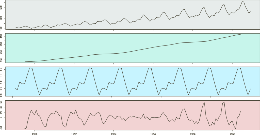
The series X, TR and CYCLE are reported in Figure $2.7$.
This is exactly the procedure that we follow in practice except that we esti-
ate parameters rather than impute them from the known DGP.
genr CYCLE $=\mathrm{X}-\mathrm{TR}$
The series X, TR and CYCLE are reported in Figure 2.7.
This is exactly the procedure that we follow in practice except that we estimate parameters rather than impute them from the known DGP.
宏观经济学代写
经济代写|宏观经济学作业代写MACROECONOMICS代考|BEVERIDGE-NELSON DECOMPOSITION OF AN一世米一种(1,1)过程
考虑这个过程:
ΔX吨=ε吨+θε吨−1,0<θ<1.
在这种情况下,我们有:
C(大号)=1+θ大号
C(1)=1+θ
C∗(大号)=C(大号)−C(1)1−大号 =−θ
BN 分解给出以下结果:
X吨=C吨+吨R吨 =−θε吨+(1+θ)和吨.
经济代写|宏观经济学作业代写MACROECONOMICS代考|BEVERIDGE-NELSON DECOMPOSITION OF AN一种R一世米一种(1,1)过程
考虑这个过程:
ΔX吨=ρΔX吨−1+ε吨+θε吨−1
在这种情况下,我们有C(大号)=1+θ大号1−ρ大号 C(1)=1+θ1−ρ C∗(大号)=C(大号)−C(1)1−大号 =−θ+ρ(1−ρ)(1−ρ大号)
BN分解给出以下结果:
X吨=C吨+吨R吨 =−θ+ρ(1−ρ)(1−ρ大号)ε吨+1+θ1−ρ和吨
经济代写|宏观经济学作业代写MACROECONOMICS代考|DERIVING THE BEVERIDGE-NELSON DECOMPOSITION IN PRACTICE
任何 ARIMA 过程的 BN 分解的实际推导很容易通过应用 Cuddington 和 Winters 建议的方法推导([6]). 对于任何我1过程中,我们已经看到随机趋势可以表示如下:
吨R吨=吨R吨−1+μ+C(1)ε吨
然后可以通过以下步骤应用分解:
- 确定适当的 ARIMA 模型并进行估计ε吨和所有参数μ和C(1)和
- 给定一个初始值吨R0采用2.13生成时间序列的永久组件
- 生成周期性分量作为每个时期的观测值与永久分量之间的差
上述程序将使永久分量达到常数,如果该程序的精度不令人满意,可以使用进一步的条件来更精确地识别分解。例如,可以施加周期性分量的样本均值为零的条件来确定永久分量中的常数。
为了说明该过程在实践中的工作原理,我们模拟了一个有马(1,1,1)通过运行以下程序,在 E-Views 中获取 200 个观察样本:
smpl 12
类型X=0
smpl 1200
genr u=nrnd
smpl 3200
系列X=X(−1)+0.6∗X(−1)−0.6∗X(−2)+在+0.5∗在(−1)
从上一节我们知道了我们的精确 BN 分解X吨:
X吨=C吨+吨R吨 =−1.1(1−0.6)(1−0.6大号)ε吨+1.50.4和吨 吨R吨=吨R吨−1+1.50.4ε吨
因此,我们可以生成永久组件X和临时组件如下:
smpl 12
genrp=0
smpl 3200
系列吨R=吨R(−1)+(1.5/0,4)∗在
smpl12
类型p=0
smpl 3200
系列吨R=吨R(−1)+(1.5/0.4)∗在
genr CYCLE=X-TR
系列 X、TR 和 CYCLE 报告在图2.7.
这正是我们在实践中遵循的过程,只是我们估计
参数而不是从已知的 DGP 中估算它们。
类型循环=X−吨R
系列 X、TR 和 CYCLE 在图 2.7 中报告。
这正是我们在实践中遵循的过程,只是我们估计参数而不是从已知的 DGP 中估算它们。

经经济代写|宏观经济学作业代写Macroeconomics代考 请认准UprivateTA™. UprivateTA™为您的留学生涯保驾护航。