如果你也在 怎样代写matlab这个学科遇到相关的难题,请随时右上角联系我们的24/7代写客服。matlab是由MathWorks公司开发的一种专有的多范式编程语言和数字计算环境。MATLAB允许进行矩阵操作、绘制函数和数据、实现算法、创建用户界面以及与用其他语言编写的程序对接。
matlab尽管MATLAB主要用于数值计算,但一个可选的工具箱使用MuPAD符号引擎,允许访问符号计算能力。一个额外的软件包,Simulink,为动态和嵌入式系统增加了图形化的多域仿真和基于模型的设计。截至2020年,MATLAB在全球拥有超过400万用户。他们来自工程、科学和经济的各种背景。
my-assignmentexpert™ matlab作业代写,免费提交作业要求, 满意后付款,成绩80\%以下全额退款,安全省心无顾虑。专业硕 博写手团队,所有订单可靠准时,保证 100% 原创。my-assignmentexpert™, 最高质量的matlab作业代写,服务覆盖北美、欧洲、澳洲等 国家。 在代写价格方面,考虑到同学们的经济条件,在保障代写质量的前提下,我们为客户提供最合理的价格。 由于统计Statistics作业种类很多,同时其中的大部分作业在字数上都没有具体要求,因此matlab作业代写的价格不固定。通常在经济学专家查看完作业要求之后会给出报价。作业难度和截止日期对价格也有很大的影响。
想知道您作业确定的价格吗? 免费下单以相关学科的专家能了解具体的要求之后在1-3个小时就提出价格。专家的 报价比上列的价格能便宜好几倍。
my-assignmentexpert™ 为您的留学生涯保驾护航 在数学Mathematics作业代写方面已经树立了自己的口碑, 保证靠谱, 高质且原创的matlab代写服务。我们的专家在数学Mathematics代写方面经验极为丰富,各种matlab相关的作业也就用不着 说。
我们提供的matlab及其相关学科的代写,服务范围广, 其中包括但不限于:
数学代写|matlab代写|Introduction
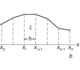
Discrete data sets, or tables of the form
\begin{tabular}{|l|l|l|l|l|}
\hline$x_{1}$ & $x_{2}$ & $x_{3}$ & $\cdots$ & $x_{n}$ \
\hline$y_{1}$ & $y_{2}$ & $y_{3}$ & $\cdots$ & $y_{n}$ \
\hline
\end{tabular}
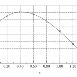
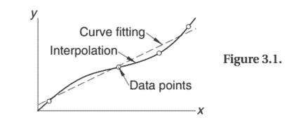
are commonly involved in technical calculations. The source of the data may be experimental observations or numerical computations. There is a distinction between interpolation and curve fitting. In interpolation we construct a curve through the data points. In doing so, we make the implicit assumption that the data points are accurate and distinct. Curve fitting is applied to data that contain scatter (noise), usually due to measurement errors. Here we want to find a smooth curve that approximates the data in some sense. Thus the curve does not have to hit the data points. This difference between interpolation and curve fitting is illustrated in Fig. 3.1.
数学代写|matlab代写|Polynomial Interpolation
Lagrange’s Method
The simplest form of an interpolant is a polynomial. It is always possible to construct a unique polynomial $P_{n-1}(x)$ of degree $n-1$ that passes through $n$ distinct data points.
One means of obtaining this polynomial is the formula of Lagrange
$$
P_{n-1}(x)=\sum_{i=1}^{n} y_{i} \ell_{i}(x)
$$
where
$$
\begin{aligned}
\ell_{i}(x) &=\frac{x-x_{1}}{x_{i}-x_{1}} \cdot \frac{x-x_{2}}{x_{i}-x_{2}} \cdots \frac{x-x_{i-1}}{x_{i}-x_{i-1}} \cdot \frac{x-x_{i+1}}{x_{i}-x_{i+1}} \cdots \frac{x-x_{n}}{x_{i}-x_{n}} \
&=\prod_{\substack{j=1 \
j \neq i}}^{n} \frac{x-x_{j}}{x_{i}-x_{j}}, \quad i=1,2, \ldots, n
\end{aligned}
$$
are called the cardinal functions.
For example, if $n=2$, the interpolant is the straight line $P_{1}(x)=y_{1} \ell_{1}(x)+y_{2} \ell_{2}(x)$, where
$$
\ell_{1}(x)=\frac{x-x_{2}}{x_{1}-x_{2}} \quad \ell_{2}(x)=\frac{x-x_{1}}{x_{2}-x_{1}}
$$
With $n=3$, interpolation is parabolic: $P_{2}(x)=y_{1} \ell_{1}(x)+y_{2} \ell_{2}(x)+y_{3} \ell_{3}(x)$, where now
$$
\begin{aligned}
&\ell_{1}(x)=\frac{\left(x-x_{2}\right)\left(x-x_{3}\right)}{\left(x_{1}-x_{2}\right)\left(x_{1}-x_{3}\right)} \
&\ell_{2}(x)=\frac{\left(x-x_{1}\right)\left(x-x_{3}\right)}{\left(x_{2}-x_{1}\right)\left(x_{2}-x_{3}\right)} \
&\ell_{3}(x)=\frac{\left(x-x_{1}\right)\left(x-x_{2}\right)}{\left(x_{3}-x_{1}\right)\left(x_{3}-x_{2}\right)}
\end{aligned}
$$
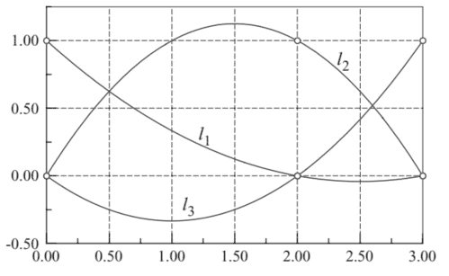
The cardinal functions are polynomials of degree $n-1$ and have the property
$$
\ell_{i}\left(x_{j}\right)=\left{\begin{array}{ll}
0 & \text { if } i \neq j \
1 & \text { if } i=j
\end{array}\right}=\delta_{i j}
$$
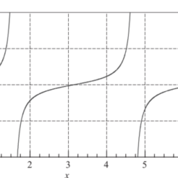
where $\delta_{i j}$ is the Kronecker delta. This property is illustrated in Fig. $3.2$ for three-point interpolation $(n=3)$ with $x_{1}=0, x_{2}=2$ and $x_{3}=3$.
数学代写|MATLAB代写|LU Decomposition Methods
It is possible to show that any square matrix A can be expressed as a product of a lower triangular matrix L and an upper triangular matrix $\mathbf{U}$ :
$$
\mathbf{A}=\mathbf{L U}
$$
The process of computing $\mathbf{L}$ and $\mathbf{U}$ for a given A is known as $L U$ decomposition or $L U$ factorization. LU decomposition is not unique (the combinations of $\mathbf{L}$ and $\mathbf{U}$ for a prescribed A are endless), unless certain constraints are placed on L or U. These constraints distinguish one type of decomposition from another. Three commonly used decompositions are listed in Table 2.2.
\begin{tabular}{|l|l|}
\hline Name & Constraints \
\hline \hline Doolittle’s decomposition & $L_{i i}=1, \quad i=1,2, \ldots, n$ \
\hline Crout’s decomposition & $U_{i i}=1, \quad i=1,2, \ldots, n$ \
\hline Choleski’s decomposition & $\mathbf{L}=\mathbf{U}^{T}$ \
\hline
\end{tabular}
Table $2.2$
After decomposing $\mathbf{A}$, it is easy to solve the equations $\mathbf{A x}=\mathbf{b}$, as pointed out in Art. 2.1. We first rewrite the equations as $\mathbf{L U x}=\mathbf{b}$. Upon using the notation $\mathbf{U x}=\mathbf{y}$, the equations become
$$
\text { Ly }=\mathbf{b}
$$
matlab代写
数学代写|MATLAB代写|INTRODUCTION
离散数据集或表格
\begin{表格}{|l|l|l|l|l|} \hline$x_{1}$ & $x_{2}$ & $x_{3}$ & $\cdots$ & $x_{n }$ \ \hline$y_{1}$ & $y_{2}$ & $y_{3}$ & $\cdots$ & $y_{n}$ \ \hline \end{表格}\begin{表格}{|l|l|l|l|l|} \hline$x_{1}$ & $x_{2}$ & $x_{3}$ & $\cdots$ & $x_{n }$ \ \hline$y_{1}$ & $y_{2}$ & $y_{3}$ & $\cdots$ & $y_{n}$ \ \hline \end{表格}
通常涉及技术计算。数据的来源可能是实验观察或数值计算。插值和曲线拟合之间存在区别。在插值中,我们通过数据点构建一条曲线。在这样做的过程中,我们隐含地假设数据点是准确和不同的。曲线拟合适用于包含散点图的数据n这一世s和,通常是由于测量误差。在这里,我们希望找到一条在某种意义上近似于数据的平滑曲线。因此曲线不必触及数据点。插值和曲线拟合之间的差异如图 3.1 所示。
数学代写|MATLAB代写|POLYNOMIAL INTERPOLATION
拉格朗日方法
最简单的插值形式是多项式。总是可以构造一个唯一的多项式磷n−1(X)学位n−1穿过n不同的数据点。
获得该多项式的一种方法是拉格朗日公式
磷n−1(X)=∑一世=1n是一世ℓ一世(X)
在哪里
ℓ一世(X)=X−X1X一世−X1⋅X−X2X一世−X2⋯X−X一世−1X一世−X一世−1⋅X−X一世+1X一世−X一世+1⋯X−XnX一世−Xn =∏j=1 j≠一世nX−XjX一世−Xj,一世=1,2,…,n
称为基函数。
例如,如果n=2, 插值是直线磷1(X)=是1ℓ1(X)+是2ℓ2(X), 在哪里
ℓ1(X)=X−X2X1−X2ℓ2(X)=X−X1X2−X1
和n=3,插值是抛物线的:磷2(X)=是1ℓ1(X)+是2ℓ2(X)+是3ℓ3(X), 现在在哪里
ℓ1(X)=(X−X2)(X−X3)(X1−X2)(X1−X3) ℓ2(X)=(X−X1)(X−X3)(X2−X1)(X2−X3) ℓ3(X)=(X−X1)(X−X2)(X3−X1)(X3−X2)
基函数是次数多项式n−1并拥有财产
\ell_{i}\left(x_{j}\right)=\left{\begin{array}{ll} 0 & \text { if } i \neq j \ 1 & \text { if } i=j \结束{数组}\right}=\delta_{i j}\ell_{i}\left(x_{j}\right)=\left{\begin{array}{ll} 0 & \text { if } i \neq j \ 1 & \text { if } i=j \结束{数组}\right}=\delta_{i j}
在哪里d一世j是克罗内克三角洲。该属性如图所示。3.2用于三点插值(n=3)和X1=0,X2=2和X3=3.
数学代写|MATLAB代写|LU DECOMPOSITION METHODS
可以证明,任何方阵 A 都可以表示为下三角矩阵 L 和上三角矩阵的乘积在 :
一种=大号在
计算过程大号和在对于给定的 A 称为大号在分解或大号在因式分解。LU分解不是唯一的吨H和C这米b一世n一种吨一世这ns这F$大号$一种nd$在$F这r一种pr和sCr一世b和d一种一种r和和ndl和ss,除非对 L 或 U 施加了某些约束。这些约束将一种分解类型与另一种分解类型区分开来。表 2.2 列出了三种常用的分解方法。
\begin{tabular}{|l|l|} \hline Name & Constraints \ \hline \hline Doolittle 的分解 & $L_{i i}=1, \quad i=1,2, \ldots, n$ \ \hline Crout’s分解 & $U_{i i}=1, \quad i=1,2, \ldots, n$ \ \hline Choleski 分解 & $\mathbf{L}=\mathbf{U}^{T}$ \ \hline \结束{表格}\begin{tabular}{|l|l|} \hline Name & Constraints \ \hline \hline Doolittle 的分解 & $L_{i i}=1, \quad i=1,2, \ldots, n$ \ \hline Crout’s分解 & $U_{i i}=1, \quad i=1,2, \ldots, n$ \ \hline Choleski 分解 & $\mathbf{L}=\mathbf{U}^{T}$ \ \hline \结束{表格}
桌子2.2
分解后一种, 很容易解方程一种X=b,正如艺术中指出的那样。2.1。我们首先将方程改写为大号在X=b. 使用符号时在X=是,方程变为

数学代写|matlab代写 请认准UprivateTA™. UprivateTA™为您的留学生涯保驾护航。