如果你也在 怎样代写数字信号处理digital signal process这个学科遇到相关的难题,请随时右上角联系我们的24/7代写客服。数字信号处理digital signal process是指使用数字处理,如通过计算机或更专业的数字信号处理器,来进行各种信号处理操作。以这种方式处理的数字信号是一连串的数字,代表时间、空间或频率等领域中连续变量的样本。在数字电子学中,数字信号被表示为脉冲序列,它通常由晶体管的开关产生。
数字信号处理digital signal process和模拟信号处理是信号处理的子领域。DSP的应用包括音频和语音处理、声纳、雷达和其他传感器阵列处理、频谱密度估计、统计信号处理、数字图像处理、数据压缩、视频编码、音频编码、图像压缩、电信的信号处理、控制系统、生物医学工程和地震学等。
my-assignmentexpert™ 数字信号处理digital signal process作业代写,免费提交作业要求, 满意后付款,成绩80\%以下全额退款,安全省心无顾虑。专业硕 博写手团队,所有订单可靠准时,保证 100% 原创。my-assignmentexpert™, 最高质量的数字信号处理digital signal process作业代写,服务覆盖北美、欧洲、澳洲等 国家。 在代写价格方面,考虑到同学们的经济条件,在保障代写质量的前提下,我们为客户提供最合理的价格。 由于统计Statistics作业种类很多,同时其中的大部分作业在字数上都没有具体要求,因此数字信号处理digital signal process作业代写的价格不固定。通常在经济学专家查看完作业要求之后会给出报价。作业难度和截止日期对价格也有很大的影响。
想知道您作业确定的价格吗? 免费下单以相关学科的专家能了解具体的要求之后在1-3个小时就提出价格。专家的 报价比上列的价格能便宜好几倍。
my-assignmentexpert™ 为您的留学生涯保驾护航 在信息Information作业代写方面已经树立了自己的口碑, 保证靠谱, 高质且原创的数字信号处理digital signal process代写服务。我们的专家在信息Information代写方面经验极为丰富,各种数字信号处理digital signal process相关的作业也就用不着 说。
我们提供的数字信号处理digital signal process及其相关学科的代写,服务范围广, 其中包括但不限于:
调和函数 harmonic function
椭圆方程 elliptic equation
抛物方程 Parabolic equation
双曲方程 Hyperbolic equation
非线性方法 nonlinear method
变分法 Calculus of Variations
几何分析 geometric analysis
偏微分方程数值解 Numerical solution of partial differential equations
信号代写|数字信号处理作业代写digital signal process代考|Classical Quantization Model
Quantization is described by Widrow’s quantization theorem [Wid61]. This says that a quantizer can be modeled (see Fig. 2.2) as the addition of a uniform distributed random signal $e(n)$ to the original signal $x(n)$ (see Fig. 2.2, [Wid61]). This additive model,
$$
x_{Q}(n)=x(n)+e(n),
$$
is based on the difference between quantized output and input according to the error signal
$$
e(n)=x_{Q}(n)-x(n) .
$$
信号代写|数字信号处理作业代写digital signal process代考|Quantization Theorem
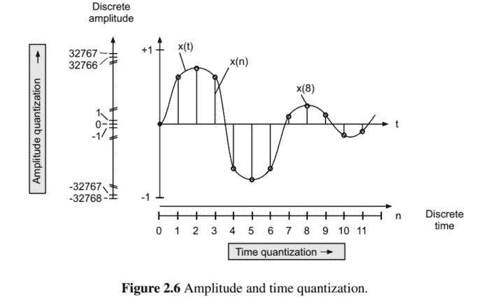
The statement of the quantization theorem for amplitude sampling (digitizing the amplitude) of signals was given by Widrow [Wid61]. The analogy for digitizing the time axis is the sampling theorem due to Shannon [Sha48]. Figure $2.6$ shows the amplitude quantization and the time quantization. First of all, the PDF of the output signal of a quantizer is determined in terms of the PDF of the input signal. Both probability density functions are shown in Fig. 2.7. The respective characteristic functions (Fourier transform of a PDF) of the input and output signals form the basis for Widrow’s quantization theorem.
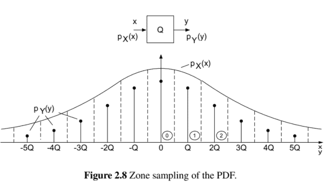
Quantization of a continuous-amplitude signal $x$ with PDF $p_{X}(x)$ leads to a discreteamplitude signal $y$ with PDF $p_{Y}(y)$ (see Fig. 2.8). The continuous PDF of the input is sampled by integrating over all quantization intervals (zone sampling). This leads to a discrete PDF of the output.
In the quantization intervals, the discrete PDF of the output is determined by the probability
$$
W[k Q]=W\left[-\frac{Q}{2}+k Q \leq x<\frac{Q}{2}+k Q\right]=\int_{-Q / 2+k Q}^{Q / 2+k Q} p_{X}(x) d x
$$
信号代写|数字信号处理作业代写digital signal process代考|Statistics of Quantization Error
The PDF of the quantization error depends on the PDF of the input and is dealt with in the following. The quantization error $e=x_{Q}-x$ is restricted to the interval $\left[-\frac{Q}{2}, \frac{Q}{2}\right]$. It depends linearly on the input (see Fig. 2.13). If the input value lies in the interval $\left[-\frac{Q}{2}, \frac{Q}{2}\right]$ then the error is $e=0-x$. For the PDF we obtain $p_{E}(e)=p_{X}(e)$. If the input value lies in the interval $\left[-\frac{Q}{2}+Q, \frac{Q}{2}+Q\right]$ then the quantization error is $e=Q\left\lfloor Q^{-1} x+0.5\right\rfloor-x$ and is again restricted to $\left[-\frac{Q}{2}, \frac{Q}{2}\right]$. The PDF of the quantization error is consequently $p_{E}(e)=p_{X}(e+Q)$ and is added to the first term. For the sum over all intervals we can write
$$
p_{E}(e)= \begin{cases}\sum_{k=-\infty}^{\infty} p_{X}(e-k Q), & -\frac{Q}{2} \leq e<\frac{Q}{2}, \ 0, & \text { elsewhere. }\end{cases}
$$
Because of the restricted values of the variable of the PDF, we can write
$$
\begin{aligned}
p_{E}(e) &=\operatorname{rect}\left(\frac{e}{Q}\right) \sum_{k=-\infty}^{\infty} p_{X}(e-k Q) \
&=\operatorname{rect}\left(\frac{e}{Q}\right)\left[p_{X}(e) * \delta_{Q}(e)\right]
\end{aligned}
$$

数字信号处理代写
信号代写|数字信号处理作业代写DIGITAL SIGNAL PROCESS代考|CLASSICAL QUANTIZATION MODEL
量化由 Widrow 量化定理描述在一世d61. 这表示可以对量化器进行建模s和和F一世G.2.2作为一个均匀分布的随机信号的添加和(n)对原始信号X(n) s和和F一世G.2.2,[在一世d61]. 这种加法模型,
X问(n)=X(n)+和(n),
是基于根据误差信号量化的输出和输入之间的差异
$$
e(n)=x_{Q}(n)-x(n) .
$$
信号代写|数字信号处理作业代写DIGITAL SIGNAL PROCESS代考|QUANTIZATION THEOREM
幅度采样量化定理的陈述d一世G一世吨一世和一世nG吨H和一种米pl一世吨在d和信号由寡妇给出在一世d61. 数字化时间轴的类比是由于香农的采样定理小号H一种48. 数字2.6显示幅度量化和时间量化。首先,量化器的输出信号的 PDF 是根据输入信号的 PDF 确定的。两个概率密度函数如图 2.7 所示。各自的特征函数F这在r一世和r吨r一种nsF这r米这F一种磷DF输入和输出信号的大小构成了 Widrow 量化定理的基础。
连续幅度信号的量化X带PDFpX(X)导致离散幅度信号是带PDFp是(是) s和和F一世G.2.8. 通过对所有量化间隔进行积分来对输入的连续 PDF 进行采样和这n和s一种米pl一世nG. 这导致输出的离散 PDF。
在量化间隔中,输出的离散 PDF 由概率决定
$$
W[k Q]=W\left[-\frac{Q}{2}+k Q \leq x<\frac{Q}{2}+k Q\right]=\int_{-Q / 2+k Q}^{Q / 2+k Q} p_{X}(x) d x
$$
信号代写|数字信号处理作业代写DIGITAL SIGNAL PROCESS代考|STATISTICS OF QUANTIZATION ERROR
量化误差的 PDF 取决于输入的 PDF 并在下面处理。量化误差和=X问−X限于区间[−问2,问2]. 它与输入线性相关s和和F一世G.2.13. 如果输入值在区间内[−问2,问2]那么错误是和=0−X. 对于我们获得的 PDFp和(和)=pX(和). 如果输入值在区间内[−问2+问,问2+问]那么量化误差是和=问⌊问−1X+0.5⌋−X并再次被限制在[−问2,问2]. 因此,量化误差的 PDF 为p和(和)=pX(和+问)并添加到第一项。对于所有区间的总和,我们可以写
p和(和)={∑ķ=−∞∞pX(和−ķ问),−问2≤和<问2, 0, 别处。
由于 PDF 变量的值受限,我们可以写
$$
\begin{aligned}
p_{E}(e) &=\operatorname{rect}\left(\frac{e}{Q}\right) \sum_{k=-\infty}^{\infty} p_{X}(e-k Q) \
&=\operatorname{rect}\left(\frac{e}{Q}\right)\left[p_{X}(e) * \delta_{Q}(e)\right]
\end{aligned}
$$

信号代写|数字信号处理作业代写digital signal process代考 请认准UprivateTA™. UprivateTA™为您的留学生涯保驾护航。