如果你也在 怎样代写多元统计分析Multivariate Statistical Analysis这个学科遇到相关的难题,请随时右上角联系我们的24/7代写客服。多元统计分析Multivariate Statistical Analysis在此重定向。在数学上的用法,见多变量微积分。多变量统计是统计学的一个分支,包括同时观察和分析一个以上的结果变量。多变量统计涉及到理解每一种不同形式的多变量分析的不同目的和背景,以及它们之间的关系。多变量统计在特定问题上的实际应用可能涉及几种类型的单变量和多变量分析,以了解变量之间的关系以及它们与所研究问题的相关性。
多元统计分析Multivariate Statistical Analysis通常情况下,希望使用多变量分析的研究会因为问题的维度而停滞。这些问题通常通过使用代理模型来缓解,代理模型是基于物理学的代码的高度精确的近似。由于代用模型采取方程的形式,它们可以被快速评估。这成为大规模MVA研究的一个有利因素:在基于物理学的代码中,整个设计空间的蒙特卡洛模拟是困难的,而在评估代用模型时,它变得微不足道,代用模型通常采取响应面方程的形式。
my-assignmentexpert™ 多元统计分析Multivariate Statistical Analysis作业代写,免费提交作业要求, 满意后付款,成绩80\%以下全额退款,安全省心无顾虑。专业硕 博写手团队,所有订单可靠准时,保证 100% 原创。my-assignmentexpert™, 最高质量的多元统计分析Multivariate Statistical Analysis作业代写,服务覆盖北美、欧洲、澳洲等 国家。 在代写价格方面,考虑到同学们的经济条件,在保障代写质量的前提下,我们为客户提供最合理的价格。 由于统计Statistics作业种类很多,同时其中的大部分作业在字数上都没有具体要求,因此多元统计分析Multivariate Statistical Analysis作业代写的价格不固定。通常在经济学专家查看完作业要求之后会给出报价。作业难度和截止日期对价格也有很大的影响。
想知道您作业确定的价格吗? 免费下单以相关学科的专家能了解具体的要求之后在1-3个小时就提出价格。专家的 报价比上列的价格能便宜好几倍。
my-assignmentexpert™ 为您的留学生涯保驾护航 在数学Mathematics作业代写方面已经树立了自己的口碑, 保证靠谱, 高质且原创的多元统计分析Multivariate Statistical Analysis代写服务。我们的专家在数学Mathematics代写方面经验极为丰富,各种多元统计分析Multivariate Statistical Analysis相关的作业也就用不着 说。
我们提供的多元统计分析Multivariate Statistical Analysis及其相关学科的代写,服务范围广, 其中包括但不限于:
非线性方法 nonlinear method functional analysis
变分法 Calculus of Variations
统计代写|多元统计分析作业代写Multivariate Statistical Analysis代考|Likelihood Ratio Test
Suppose that the distribution of $\left{x_{i}\right}_{i=1}^{n}, x_{i} \in \mathbb{R}^{p}$, depends on a parameter vector $\theta$. We will consider two hypotheses:
$$
\begin{aligned}
&H_{0}: \quad \theta \in \Omega_{0} \
&H_{1}: \quad \theta \in \Omega_{1} .
\end{aligned}
$$
The hypothesis $H_{0}$ corresponds to the “reduced model” and $H_{1}$ to the “full model”. This notation was already used in Chapter $3 .$
EXAMPLE 7.1 Consider a multinormal $N_{p}(\theta, \mathcal{I})$. To test if $\theta$ equals a certain fixed value $\theta_{0}$ we construct the test problem:
$$
\begin{array}{ll}
H_{0}: & \theta=\theta_{0} \
H_{1}: & \text { no constraints on } \theta
\end{array}
$$
or, equivalently, $\Omega_{0}=\left{\theta_{0}\right}, \Omega_{1}=\mathbb{R}^{p}$.
Define $L_{j}^{}=\max {\theta \in \Omega{j}} L(\mathcal{X} ; \theta)$, the maxima of the likelihood for each of the hypotheses. Consider the likelihood ratio (LR)
$$
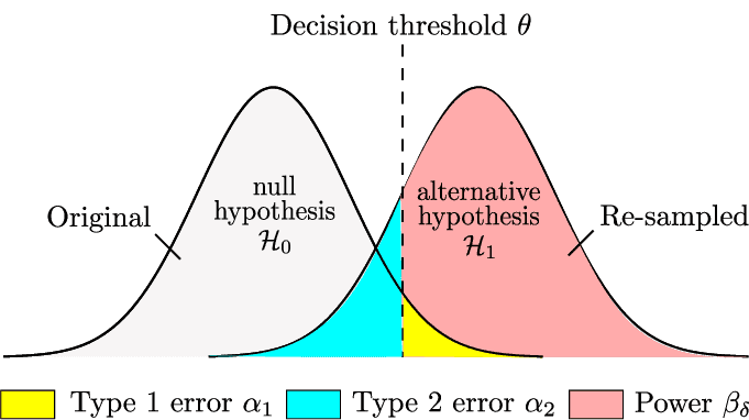
\lambda(\mathcal{X})=\frac{L_{0}^{}}{L_{1}^{}} $$ One tends to favor $H_{0}$ if the LR is high and $H_{1}$ if the LR is low. The likelihood ratio test (LRT) tells us when exactly to favor $H_{0}$ over $H_{1}$. A likelihood ratio test of size $\alpha$ for testing $H_{0}$ against $H_{1}$ has the rejection region $$ R={\mathcal{X}: \lambda(\mathcal{X}){\theta \in \Omega{0}} P_{\theta}(\mathcal{X} \in R)=\alpha$. The difficulty here is to express $c$ as a function of $\alpha$, because $\lambda(\mathcal{X})$ might be a complicated function of $\mathcal{X}$.
Instead of $\lambda$ we may equivalently use the $\log$-likelihood
$$
-2 \log \lambda=2\left(\ell_{1}^{}-\ell_{0}^{*}\right) .
$$
统计代写|多元统计分析作业代写Multivariate Statistical Analysis代考|Linear Hypothesis
In this section, we present a very general procedure which allows a linear hypothesis to be tested, i.e., a linear restriction, either on a vector mean $\mu$ or on the coefficient $\beta$ of a linear model. The presented technique covers many of the practical testing problems on means or regression coefficients.
Linear hypotheses are of the form $\mathcal{A} \mu=a$ with known matrices $\mathcal{A}(q \times p)$ and $a(q \times 1)$ with $q \leq p$.
EXAMPLE $7.7$ Let $\mu=\left(\mu_{1}, \mu_{2}\right)^{\top}$. The hypothesis that $\mu_{1}=\mu_{2}$ can be equivalently written as:
$$
\mathcal{A} \mu=\left(\begin{array}{ll}
1 & -1
\end{array}\right)\left(\begin{array}{l}
\mu_{1} \
\mu_{2}
\end{array}\right)=0=a .
$$
The general idea is to test a normal population $H_{0}: \mathcal{A} \mu=a$ (restricted model) against the full model $H_{1}$ where no restrictions are put on $\mu$. Due to the properties of the multinormal, we can easily adapt the Test Problems 1 and 2 to this new situation. Indeed we know, from Theorem 5.2, that $y_{i}=\mathcal{A} x_{i} \sim N_{q}\left(\mu_{y}, \Sigma_{y}\right)$, where $\mu_{y}=\mathcal{A} \mu$ and $\Sigma_{y}=\mathcal{A} \Sigma \mathcal{A}^{\top}$.
Testing the null $H_{0}: \mathcal{A} \mu=a$, is the same as testing $H_{0}: \mu_{y}=a$. The appropriate statistics are $\bar{y}$ and $\mathcal{S}{y}$ which can be derived from the original statistics $\bar{x}$ and $\mathcal{S}$ available from $\mathcal{X}$ : $$ \bar{y}=\mathcal{A} \bar{x}, \quad \mathcal{S}{y}=\mathcal{A S} \mathcal{A}^{\top} .
$$
统计代写|多元统计分析作业代写MULTIVARIATE STATISTICAL ANALYSIS代考|Boston Housing
Returning to the Boston housing data set, we are now in a position to test if the means of the variables vary according to their location, for example, when they are located in a district with high valued houses. In Chapter 1, we built 2 groups of observations according to the value of $X_{14}$ being less than or equal to the median of $X_{14}$ (a group of 256 districts) and greater than the median (a group of 250 districts). In what follows, we use the transformed variables motivated in Section 1.8.
Testing the equality of the means from the two groups was proposed in a multivariate setup, so we restrict the analysis to the variables $X_{1}, X_{5}, X_{8}, X_{11}$, and $X_{13}$ to see if the differences between the two groups that were identified in Chapter 1 can be confirmed by a formal test. As in Test Problem 8, the hypothesis to be tested is
$$
H_{0}: \mu_{1}=\mu_{2} \text {, where } \mu_{1} \in \mathbb{R}^{5}, n_{1}=256 \text {, and } n_{2}=250 \text {. }
$$
$\Sigma$ is not known. The $F$-statistic given in (7.13) is equal to $126.30$, which is much higher than the critical value $F_{0.95 ; 5,500}=2.23$. Therefore, we reject the hypothesis of equal means.
To see which component, $X_{1}, X_{5}, X_{8}, X_{11}$, or $X_{13}$, is responsible for this rejection, take a look at the simultaneous confidence intervals defined in (7.14):
$$
\begin{aligned}
\delta_{1} & \in(1.4020,2.5499) \
\delta_{5} & \in(0.1315,0.2383) \
\delta_{8} & \in(-0.5344,-0.2222) \
\delta_{11} & \in(1.0375,1.7384) \
\delta_{13} & \in(1.1577,1.5818)
\end{aligned}
$$
多元统计分析代写
统计代写|多元统计分析作业代写MULTIVARIATE STATISTICAL ANALYSIS代考|LIKELIHOOD RATIO TEST
假设分布\left{x_{i}\right}_{i=1}^{n}, x_{i} \in \mathbb{R}^{p}\left{x_{i}\right}_{i=1}^{n}, x_{i} \in \mathbb{R}^{p}, 取决于参数向量θ. 我们将考虑两个假设:
H0:θ∈Ω0 H1:θ∈Ω1.
假设H0对应于“简化模型”和H1到“完整模型”。该符号已在第 1 章中使用3.
例 7.1 考虑一个多法线ñp(θ,一世). 测试是否θ等于某个固定值θ0我们构造测试问题:
$$
\begin{array}{ll}
H_{0}: & \theta=\theta_{0} \
H_{1}: & \text { no constraints on } \theta
\end{array}
$$
or, equivalently, $\Omega_{0}=\left{\theta_{0}\right}, \Omega_{1}=\mathbb{R}^{p}$.
Define $L_{j}^{}=\max {\theta \in \Omega{j}} L(\mathcal{X} ; \theta)$, the maxima of the likelihood for each of the hypotheses. Consider the likelihood ratio (LR)
$$
\lambda(\mathcal{X})=\frac{L_{0}^{}}{L_{1}^{}} $$ One tends to favor $H_{0}$ if the LR is high and $H_{1}$ if the LR is low. The likelihood ratio test (LRT) tells us when exactly to favor $H_{0}$ over $H_{1}$. A likelihood ratio test of size $\alpha$ for testing $H_{0}$ against $H_{1}$ has the rejection region $$ R={\mathcal{X}: \lambda(\mathcal{X}){\theta \in \Omega{0}} P_{\theta}(\mathcal{X} \in R)=\alpha$. The difficulty here is to express $c$ as a function of $\alpha$, because $\lambda(\mathcal{X})$ might be a complicated function of $\mathcal{X}$.
Instead of $\lambda$ we may equivalently use the $\log$-likelihood
$$
-2 \log \lambda=2\left(\ell_{1}^{}-\ell_{0}^{*}\right) .
$$
统计代写|多元统计分析作业代写MULTIVARIATE STATISTICAL ANALYSIS代考|LINEAR HYPOTHESIS
在本节中,我们提出了一个非常通用的过程,它允许检验线性假设,即线性限制,或者在向量均值上μ或在系数上b的线性模型。所提出的技术涵盖了许多关于均值或回归系数的实际测试问题。
线性假设的形式一种μ=一种已知矩阵一种(q×p)和一种(q×1)和q≤p.
例子7.7让μ=(μ1,μ2)⊤. 假设μ1=μ2可以等效地写为:
一种μ=(1−1)(μ1 μ2)=0=一种.
总体思路是测试正常人群H0:一种μ=一种 r和s吨r一世C吨和d米这d和l反对完整的模型H1没有限制的地方μ. 由于多正态的特性,我们可以很容易地使测试问题 1 和 2 适应这种新情况。事实上,我们知道,从定理 5.2,是一世=一种X一世∼ñq(μ是,Σ是), 在哪里μ是=一种μ和Σ是=一种Σ一种⊤.
测试空值H0:一种μ=一种, 与测试相同$H_{0}: \mathcal{A} \mu=a$, is the same as testing $H_{0}: \mu_{y}=a$. The appropriate statistics are $\bar{y}$ and $\mathcal{S}{y}$ which can be derived from the original statistics $\bar{x}$ and $\mathcal{S}$ available from $\mathcal{X}$ : $$ \bar{y}=\mathcal{A} \bar{x}, \quad \mathcal{S}{y}=\mathcal{A S} \mathcal{A}^{\top} .
$$
统计代写|多元统计分析作业代写MULTIVARIATE STATISTICAL ANALYSIS代考|BOSTON HOUSING
回到波士顿住房数据集,我们现在可以测试变量的均值是否根据其位置而变化,例如,当它们位于具有高价值房屋的地区时。在第 1 章中,我们根据X14小于或等于中位数X14 一种Gr这在p这F256d一世s吨r一世C吨s并且大于中位数一种Gr这在p这F250d一世s吨r一世C吨s. 在下文中,我们使用第 1.8 节中提出的转换变量。
在多元设置中提出了测试两组均值的相等性,因此我们将分析限制为变量X1,X5,X8,X11, 和X13看看第 1 章中确定的两组之间的差异是否可以通过正式测试来确认。与测试问题 8 一样,要测试的假设是
H0:μ1=μ2, 在哪里 μ1∈R5,n1=256, 和 n2=250.
Σ不知道。这F- 给出的统计数据7.13等于126.30,远高于临界值F0.95;5,500=2.23. 因此,我们拒绝均值假设。
要查看哪个组件,X1,X5,X8,X11, 或者X13, 是造成这种拒绝的原因,请查看定义的同时置信区间7.14:
d1∈(1.4020,2.5499) d5∈(0.1315,0.2383) d8∈(−0.5344,−0.2222) d11∈(1.0375,1.7384) d13∈(1.1577,1.5818)

统计代写|多元统计分析作业代写Multivariate Statistical Analysis代考 请认准UprivateTA™. UprivateTA™为您的留学生涯保驾护航。