如果你也在 怎样代写差分方程difference equation这个学科遇到相关的难题,请随时右上角联系我们的24/7代写客服。差分方程difference equation包含一个或多个导数的数学语句,即代表连续变化的量的变化率的条款。微分方程在科学和工程以及许多其他定量研究领域非常常见,因为对于正在发生变化的系统,可以直接观察和测量其变化率。
差分方程difference equation一般来说,微分方程的解是一个表达一个变量对一个或多个变量的函数依赖的方程;它通常包含原始微分方程中没有的常数项。另一种说法是,微分方程的解产生一个函数,可以用来预测原始系统的行为,至少在某些约束条件下。
my-assignmentexpert™ 差分方程difference equation作业代写,免费提交作业要求, 满意后付款,成绩80\%以下全额退款,安全省心无顾虑。专业硕 博写手团队,所有订单可靠准时,保证 100% 原创。my-assignmentexpert™, 最高质量的差分方程difference equation作业代写,服务覆盖北美、欧洲、澳洲等 国家。 在代写价格方面,考虑到同学们的经济条件,在保障代写质量的前提下,我们为客户提供最合理的价格。 由于统计Statistics作业种类很多,同时其中的大部分作业在字数上都没有具体要求,因此差分方程difference equation作业代写的价格不固定。通常在经济学专家查看完作业要求之后会给出报价。作业难度和截止日期对价格也有很大的影响。
想知道您作业确定的价格吗? 免费下单以相关学科的专家能了解具体的要求之后在1-3个小时就提出价格。专家的 报价比上列的价格能便宜好几倍。
my-assignmentexpert™ 为您的留学生涯保驾护航 在数学Mathematics作业代写方面已经树立了自己的口碑, 保证靠谱, 高质且原创的数学Mathematics代写服务。我们的专家在差分方程difference equation代写方面经验极为丰富,各种差分方程difference equation相关的作业也就用不着 说。
我们提供的差分方程difference equation及其相关学科的代写,服务范围广, 其中包括但不限于:
数学代写|差分方程作业代写difference equation代考|SCALAR INITIAL VALUE PROBLEMS
A special case of an initial value problem is when the number of dimension $n$ in the initial value problem (6.11)-(6.12) is equal to 1 . In this case we speak of a scalar problem and it is useful to study these problems if one wishes to get some insights into how finite difference methods work. A numerical and computational discussion of scalar IVP is given in Duffy (2004). In this section we discuss some numerical properties of one-step finite difference schemes for the linear scalar problem:
$$
\begin{aligned}
&L u \equiv \frac{\mathrm{d} u}{\mathrm{~d} t}+a(t) u=f(t), \quad 00, \quad \forall t \in[0, T]$
The reader can check that the one-step methods (equations (6.17), (6.18) and (6.19)) can be cast as the general form recurrence relation
$$
U^{n+1}=A^{n} U^{n}+B^{n}, \quad n \geq 0
$$
Then, using this formula and mathematical induction we can give an explicit solution at any time level as follows:
$$
U^{n}=\left(\prod_{j=0}^{n-1} A^{j}\right) U^{0}+\sum_{v=0}^{n-1} B^{v} \prod_{j=v+1}^{n-1} A^{j}, \quad n \geq 1 \quad \text { with } \prod_{j=I}^{j=J} g^{j} \equiv 1 \text { if } I>J
$$
A special case is when the coefficients $A$ and $B$ are constant, that is:
$$
U^{n+1}=A U^{n}+B, \quad n \geq 0
$$
Then the general solution is given by
$$
U^{n}=A^{n} U^{0}+B \frac{1-A^{n}}{1-A}, \quad n \geq 0
$$
where in equation (6.52) we note that $A^{n} \equiv n^{t h}$ power of constant $A$ and $A \neq 1$.
The proof of this requires the formula for the sum of a series
$$
1+A+\cdots+A^{n}=\frac{1-A^{n+1}}{1-A}, \quad A \neq 1
$$
For a readable introduction to difference schemes we refer the reader to Goldberg (1986). Learning finite difference theory for the Black-Scholes equation involves not only understanding the main concepts but also developing skills in basic arithmetic. This is absolutely vital if you wish to become proficient in this area of numerical analysis.
数学代写|差分方程作业代写difference equation代考|Exponentially fitted schemes
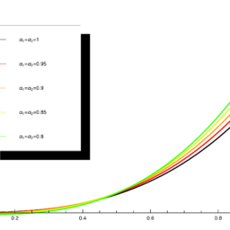
We now introduce a special class of schemes that prove to be very useful in approximating the solution of the Black-Scholes PDE. In particular, these so-called exponentially fitted schemes are able to handle discontinuities (near a strike price and at barriers, for example). In general, a fitted scheme is a modification of the Crank-Nicolson scheme (see equation (6.19)) except that we introduce a new coefficient into the difference equation. In order to find this coefficient we argue as follows: Consider the trivial IVP
$\frac{\mathrm{d} u}{\mathrm{~d} t}+a u=0, \quad a>0$ constant $u(0)=A$ with solution $u(t)=A \mathrm{e}^{-a t}$ $\sigma \frac{U^{n+1}-U^{n}}{k}+a \frac{U^{n+1}+U^{n}}{2}=0$ $U^{0}=A$
We now demand that the solution of (6.55) should equal the solution of (6.54) at the mesh points. This will determine the value of $\sigma$, and some arithmetic shows that
$$
\sigma=\frac{a k}{2} \operatorname{coth} \frac{a k}{2}
$$
where $\quad \operatorname{coth} x=\left(\mathrm{e}^{2 x}+1\right) /\left(\mathrm{e}^{2 x}-1\right)$.
This is the famous fitting factor and it has been known since the 1950 s (de Allen and Southwell, 1955), elaborated upon by Soviet scientists (Il’in, 1969) and generalised to convection-diffusion equations in Duffy (1980). Based on the fitting factor defined in equation (6.56), we propose the generalised finite difference scheme when the coefficient $a$ in equation (6.54) is variable $a=a(t)$ and non-zero right-hand side $f=f(t)$ :
$\sigma^{n} \frac{U^{n+1}-U^{n}}{k}+a^{n+\frac{1}{2}} \frac{U^{n+1}+U^{n}}{2}=f^{n+\frac{1}{2}}, \quad n \geq 0$
$u^{0}=A$
$\sigma^{n} \equiv \frac{a^{n+\frac{1}{2}} k}{2} \operatorname{coth} \frac{a^{n+\frac{1}{2}} k}{2}$
A full discussion of this scheme, its applicability to the Black-Scholes equations and its implementation in $\mathrm{C}++$ is given in Duffy (2004). We shall also reuse this fitting factor finite difference schemes for the Black-Scholes equation in later chapters in this book.
差分方程代写
数学代写|差分方程作业代写DIFFERENCE EQUATION代考|SCALAR INITIAL VALUE PROBLEMS
初始值问题的一个特例是当维数n在初值问题6.11-6.12等于 1 。在这种情况下,我们谈到了一个标量问题,如果希望了解有限差分方法的工作原理,研究这些问题是有用的。Duffy 中给出了标量 IVP 的数值和计算讨论2004. 在本节中,我们讨论线性标量问题的一步有限差分格式的一些数值性质:
$$
\begin{aligned}
&L u \equiv \frac{\mathrm{d} u}{\mathrm{~d} t}+a(t) u=f(t), \quad 00, \quad \forall t \in[0, T]$
The reader can check that the one-step methods (equations (6.17), (6.18) and (6.19)) can be cast as the general form recurrence relation
$$
U^{n+1}=A^{n} U^{n}+B^{n}, \quad n \geq 0
$$
Then, using this formula and mathematical induction we can give an explicit solution at any time level as follows:
$$
U^{n}=\left(\prod_{j=0}^{n-1} A^{j}\right) U^{0}+\sum_{v=0}^{n-1} B^{v} \prod_{j=v+1}^{n-1} A^{j}, \quad n \geq 1 \quad \text { with } \prod_{j=I}^{j=J} g^{j} \equiv 1 \text { if } I>J
$$
A special case is when the coefficients $A$ and $B$ are constant, that is:
$$
U^{n+1}=A U^{n}+B, \quad n \geq 0
$$
Then the general solution is given by
$$
U^{n}=A^{n} U^{0}+B \frac{1-A^{n}}{1-A}, \quad n \geq 0
$$
where in equation (6.52) we note that $A^{n} \equiv n^{t h}$ power of constant $A$ and $A \neq 1$.
The proof of this requires the formula for the sum of a series
$$
1+A+\cdots+A^{n}=\frac{1-A^{n+1}}{1-A}, \quad A \neq 1
$$
对于差分方案的可读介绍,我们参考读者到戈德堡1986. 学习 Black-Scholes 方程的有限差分理论不仅涉及理解主要概念,还涉及发展基本算术技能。如果您希望精通这一数值分析领域,这绝对是至关重要的。
数学代写|差分方程作业代写DIFFERENCE EQUATION代考|EXPONENTIALLY FITTED SCHEMES
我们现在介绍一类特殊的方案,它们被证明在近似 Black-Scholes PDE 的解中非常有用。特别是,这些所谓的指数拟合方案能够处理不连续性n和一种r一种s吨r一世ķ和pr一世C和一种nd一种吨b一种rr一世和rs,F这r和X一种米pl和. 一般来说,拟合方案是对 Crank-Nicolson 方案的修改s和和和q在一种吨一世这n(6.19) 除了我们在差分方程中引入了一个新系数。为了找到这个系数,我们争论如下:考虑微不足道的 IVP
d在 d吨+一种在=0,一种>0持续的在(0)=一种有溶液在(吨)=一种和−一种吨 σ在n+1−在nķ+一种在n+1+在n2=0 在0=一种
我们现在要求解决6.55应该等于解决方案6.54在网格点。这将决定σ, 一些算术表明
σ=一种ķ2考特一种ķ2
在哪里考特X=(和2X+1)/(和2X−1).
这是著名的拟合因子,自 1950 年代以来就为人所知d和一种ll和n一种nd小号这在吨H在和ll,1955,由苏联科学家详细阐述一世l′一世n,1969并推广到 Duffy 中的对流扩散方程1980. 基于方程中定义的拟合因子6.56,我们提出了广义有限差分格式,当系数一种在等式中6.54是可变的一种=一种(吨)和非零右手边F=F(吨) :
σn在n+1−在nķ+一种n+12在n+1+在n2=Fn+12,n≥0
在0=一种
σn≡一种n+12ķ2考特一种n+12ķ2
对该方案的全面讨论,它对 Black-Scholes 方程的适用性及其在C++在达菲中给出2004. 我们还将在本书后面的章节中为 Black-Scholes 方程重用这种拟合因子有限差分格式。

数学代写|差分方程作业代写difference equation代考 请认准UprivateTA™. UprivateTA™为您的留学生涯保驾护航。
微观经济学代写
微观经济学是主流经济学的一个分支,研究个人和企业在做出有关稀缺资源分配的决策时的行为以及这些个人和企业之间的相互作用。my-assignmentexpert™ 为您的留学生涯保驾护航 在数学Mathematics作业代写方面已经树立了自己的口碑, 保证靠谱, 高质且原创的数学Mathematics代写服务。我们的专家在图论代写Graph Theory代写方面经验极为丰富,各种图论代写Graph Theory相关的作业也就用不着 说。
线性代数代写
线性代数是数学的一个分支,涉及线性方程,如:线性图,如:以及它们在向量空间和通过矩阵的表示。线性代数是几乎所有数学领域的核心。
博弈论代写
现代博弈论始于约翰-冯-诺伊曼(John von Neumann)提出的两人零和博弈中的混合策略均衡的观点及其证明。冯-诺依曼的原始证明使用了关于连续映射到紧凑凸集的布劳威尔定点定理,这成为博弈论和数学经济学的标准方法。在他的论文之后,1944年,他与奥斯卡-莫根斯特恩(Oskar Morgenstern)共同撰写了《游戏和经济行为理论》一书,该书考虑了几个参与者的合作游戏。这本书的第二版提供了预期效用的公理理论,使数理统计学家和经济学家能够处理不确定性下的决策。
微积分代写
微积分,最初被称为无穷小微积分或 “无穷小的微积分”,是对连续变化的数学研究,就像几何学是对形状的研究,而代数是对算术运算的概括研究一样。
它有两个主要分支,微分和积分;微分涉及瞬时变化率和曲线的斜率,而积分涉及数量的累积,以及曲线下或曲线之间的面积。这两个分支通过微积分的基本定理相互联系,它们利用了无限序列和无限级数收敛到一个明确定义的极限的基本概念 。
计量经济学代写
什么是计量经济学?
计量经济学是统计学和数学模型的定量应用,使用数据来发展理论或测试经济学中的现有假设,并根据历史数据预测未来趋势。它对现实世界的数据进行统计试验,然后将结果与被测试的理论进行比较和对比。
根据你是对测试现有理论感兴趣,还是对利用现有数据在这些观察的基础上提出新的假设感兴趣,计量经济学可以细分为两大类:理论和应用。那些经常从事这种实践的人通常被称为计量经济学家。
Matlab代写
MATLAB 是一种用于技术计算的高性能语言。它将计算、可视化和编程集成在一个易于使用的环境中,其中问题和解决方案以熟悉的数学符号表示。典型用途包括:数学和计算算法开发建模、仿真和原型制作数据分析、探索和可视化科学和工程图形应用程序开发,包括图形用户界面构建MATLAB 是一个交互式系统,其基本数据元素是一个不需要维度的数组。这使您可以解决许多技术计算问题,尤其是那些具有矩阵和向量公式的问题,而只需用 C 或 Fortran 等标量非交互式语言编写程序所需的时间的一小部分。MATLAB 名称代表矩阵实验室。MATLAB 最初的编写目的是提供对由 LINPACK 和 EISPACK 项目开发的矩阵软件的轻松访问,这两个项目共同代表了矩阵计算软件的最新技术。MATLAB 经过多年的发展,得到了许多用户的投入。在大学环境中,它是数学、工程和科学入门和高级课程的标准教学工具。在工业领域,MATLAB 是高效研究、开发和分析的首选工具。MATLAB 具有一系列称为工具箱的特定于应用程序的解决方案。对于大多数 MATLAB 用户来说非常重要,工具箱允许您学习和应用专业技术。工具箱是 MATLAB 函数(M 文件)的综合集合,可扩展 MATLAB 环境以解决特定类别的问题。可用工具箱的领域包括信号处理、控制系统、神经网络、模糊逻辑、小波、仿真等。