如果你也在 怎样代写微分方程differential equation这个学科遇到相关的难题,请随时右上角联系我们的24/7代写客服。微分方程differential equation在数学中,是将一个或多个未知函数及其导数联系起来的方程。在应用中,函数通常代表物理量,导数代表其变化率,而微分方程则定义了两者之间的关系。这种关系很常见;因此,微分方程在许多学科,包括工程、物理学、经济学和生物学中发挥着突出作用。
微分方程differential equation研究主要包括研究其解(满足每个方程的函数集合),以及研究其解的性质。只有最简单的微分方程可以用明确的公式求解;然而,一个给定的微分方程的解的许多属性可以在不精确计算的情况下确定。
my-assignmentexpert™ 微分方程differential equation作业代写,免费提交作业要求, 满意后付款,成绩80\%以下全额退款,安全省心无顾虑。专业硕 博写手团队,所有订单可靠准时,保证 100% 原创。my-assignmentexpert™, 最高质量的微分方程differential equation作业代写,服务覆盖北美、欧洲、澳洲等 国家。 在代写价格方面,考虑到同学们的经济条件,在保障代写质量的前提下,我们为客户提供最合理的价格。 由于统计Statistics作业种类很多,同时其中的大部分作业在字数上都没有具体要求,因此微分方程differential equation作业代写的价格不固定。通常在经济学专家查看完作业要求之后会给出报价。作业难度和截止日期对价格也有很大的影响。
想知道您作业确定的价格吗? 免费下单以相关学科的专家能了解具体的要求之后在1-3个小时就提出价格。专家的 报价比上列的价格能便宜好几倍。
my-assignmentexpert™ 为您的留学生涯保驾护航 在数学mathematics作业代写方面已经树立了自己的口碑, 保证靠谱, 高质且原创的微分方程differential equation代写服务。我们的专家在数学mathematics代写方面经验极为丰富,各种微分方程differential equation相关的作业也就用不着 说。
我们提供的微分方程differential equation及其相关学科的代写,服务范围广, 其中包括但不限于:
数学代写|微分方程代写differential equation代考|Measures to increase efficiency
Although fixed-step algorithms are mainly taught in the courses such as numerical analysis, almost nobody uses them in practice, since there are too many limitations. If one wants to increase the efficiency in solving differential equations, the following measures can be considered:
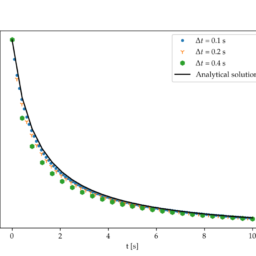
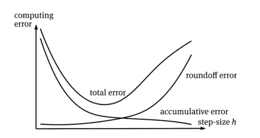
(1) Selecting a suitable step-size. As in the case of Euler’s method, the step-size should be properly chosen. It should not be too small or too large.
(2) Improving the accuracy of the algorithm. Since the accuracy of Euler’s method is too low, better algorithms should be selected. For instance, the fourth-order Runge-Kutta algorithm is a better choice.(3) Using variable-step mechanism. The “suitable” step-size mentioned earlier is a vague concept. In fact, many variable-step algorithms are available, which allow changing the step-size adaptively. When the error is small, a larger step-size can be automatically chosen to increase the speed, while when the error is too large, a smaller step-size is adopted to ensure the accuracy. Variable-step algorithms are the top choice in solving differential equations.
数学代写|微分方程代写differential equation代考|An introduction to variable-step algorithms
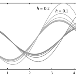
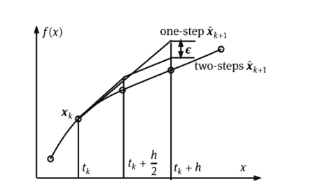
The principles of some of the variable-step algorithms are illustrated in Figure 3.4. If the state vector $\boldsymbol{x}{k}$ at time $t{k}$ is known, the initial step-size $h$ can be used to compute the state $\tilde{\boldsymbol{x}}{k+1}$ at time $t{k}+h$. On the other hand, the step-size can be reduced by half such that the state vector at $\hat{\boldsymbol{x}}{k+1}$ can be evaluated in two steps. If the error using the two step-sizes $\boldsymbol{\epsilon}=\left|\hat{\boldsymbol{x}}{k+1}-\tilde{\boldsymbol{x}}_{k+1}\right|$ is smaller than the prespecified error tolerance, the step-size can be used, or increased; if the error is too large, the step-size should be reduced, and checked again. An adaptive variable-step algorithm monitors the error in the solution process, and adjusts the step-size whenever necessary, to ensure fast speed and high accuracy.
数学代写|微分方程代写DIFFERENTIAL EQUATION代考|The 4/5th order Runge–Kutta variable-step algorithm
Erwin Felhberg, a researcher working for NASA, improved the classical Runge-Kutta method, ${ }^{[25]}$ where within each computation step, the $f_{i}(\cdot)$ function is evaluated 6 times, so as to ensure high precision and numerical stability. The efficiency of the algorithm is high and the accuracy can be controlled by the user. Therefore it is usually used in practical applications.
Theorem 3.11. Assuming that the current step-size is $h_{k}, 6$ immediate variables $\boldsymbol{k}{i}$ are evaluated as $$ \boldsymbol{k}{i}=\boldsymbol{f}\left(t_{k}+\alpha_{i} h_{k}, \boldsymbol{x}{k}+\sum{j=1}^{i-1} \beta_{i j} \boldsymbol{k}{j}\right), \quad i=1,2, \ldots, 6 $$ where $t{k}$ is the current time, and the coefficients $\alpha_{i}, \beta_{i j}$, and $\gamma_{i}$ are shown in Table 3.2. The coefficients $\alpha_{i}$ and $\beta_{i j}$ are also referred to as Dormand-Prince pairs. The state variable in the next step can be computed from
$$
\boldsymbol{x}{k+1}=\boldsymbol{x}{k}+\sum_{i=1}^{6} y_{i} h_{k} \boldsymbol{k}_{\boldsymbol{i}}
$$
微分方程代写
数学代写|微分方程代写DIFFERENTIAL EQUATION代考|MEASURES TO INCREASE EFFICIENCY
虽然固定步长算法主要在数值分析等课程中讲授,但由于存在太多限制,几乎没有人在实践中使用它们。如果想提高求解微分方程的效率,可以考虑以下措施:
1选择合适的步长。如在欧拉的方法的情况下,应正确选择阶梯大小。它不应该太小或太大。
2提高算法的准确性。由于欧拉法的精度太低,应该选择更好的算法。例如,四阶 Runge-Kutta 算法是更好的选择。3使用可变步长机制。前面提到的“合适”步长是一个模糊的概念。事实上,许多可变步长算法是可用的,它们允许自适应地改变步长。当误差较小时,可以自动选择较大的步长来提高速度,而当误差太大时,采用较小的步长来保证精度。变步长算法是求解微分方程的首选。
数学代写|微分方程代写DIFFERENTIAL EQUATION代考|AN INTRODUCTION TO VARIABLE-STEP ALGORITHMS
一些可变步长算法的原理如图 3.4 所示。如果状态向量 $\boldsymbol{x} {k}一种吨吨一世米和t {k}一世s到n这在n,吨H和一世n一世吨一世一种一世s吨和p−s一世和和HC一种nb和你s和d吨这C这米p你吨和吨H和s吨一种吨和\波浪号{\boldsymbol{x}} {k+1}一种吨吨一世米和t {k}+h.这n吨H和这吨H和rH一种nd,吨H和s吨和p−s一世和和C一种nb和r和d你C和db是H一种一世Fs你CH吨H一种吨吨H和s吨一种吨和v和C吨这r一种吨\hat{\boldsymbol{x}} {k+1}C一种nb和和v一种一世你一种吨和d一世n吨在这s吨和ps.一世F吨H和和rr这r你s一世nG吨H和吨在这s吨和p−s一世和和s\boldsymbol{\epsilon}=\left|\hat{\boldsymbol{x}} {k+1}-\tilde{\boldsymbol{x}}_{k+1}\right|$ 小于预先指定的错误公差,步长可以使用,也可以增加;如果误差过大,应减小步长,重新检查。自适应变步长算法监测求解过程中的误差,并在必要时调整步长,以确保快速和高精度。
数学代写|微分方程代写DIFFERENTIAL EQUATION代考|THE 4/5TH ORDER RUNGE–KUTTA VARIABLE-STEP ALGORITHM
为 NASA 工作的研究员 Erwin Felhberg 改进了经典的 Runge-Kutta 方法,[25]在每个计算步骤中,F一世(⋅)函数进行了6次评估,以确保高精度和数值稳定性。该算法效率高,精度可由用户控制。因此,它通常用于实际应用中。
定理 3.11。假设当前步长为H到,6直接变量 $h_{k}, 6$ immediate variables $\boldsymbol{k}{i}$ are evaluated as $$ \boldsymbol{k}{i}=\boldsymbol{f}\left(t_{k}+\alpha_{i} h_{k}, \boldsymbol{x}{k}+\sum{j=1}^{i-1} \beta_{i j} \boldsymbol{k}{j}\right), \quad i=1,2, \ldots, 6 $$ where $t{k}$ is the current time, and the coefficients $\alpha_{i}, \beta_{i j}$, and $\gamma_{i}$ are shown in Table 3.2. The coefficients $\alpha_{i}$ and $\beta_{i j}$ are also referred to as Dormand-Prince pairs. The state variable in the next step can be computed from
$$
\boldsymbol{x}{k+1}=\boldsymbol{x}{k}+\sum_{i=1}^{6} y_{i} h_{k} \boldsymbol{k}_{\boldsymbol{i}}
$$

数学代写|微分方程代写differential equation代考 请认准UprivateTA™. UprivateTA™为您的留学生涯保驾护航。