
如果你也在 怎样代写matlab这个学科遇到相关的难题,请随时右上角联系我们的24/7代写客服。matlab是由数学家和计算机程序员Cleve Moler发明的。MATLAB的想法是基于他1960年代的博士论文。Moler成为新墨西哥大学的一名数学教授,并开始为他的学生开发MATLAB 作为一种爱好。他在1967年与他曾经的论文导师George Forsythe开发了MATLAB的初始线性代数编程。随后在1971年为线性方程编写Fortran代码。
matlab的第一个早期版本是在20世纪70年代末完成的。1979年2月,该软件在加利福尼亚州的海军研究生院首次向公众披露。 MATLAB的早期版本是简单的矩阵计算器,有71个预置函数。当时,MATLAB被免费分发到各大学。Moler会在他访问的大学留下拷贝,该软件在大学校园的数学系中培养了一批强大的追随者。
my-assignmentexpert™ matlab作业代写,免费提交作业要求, 满意后付款,成绩80\%以下全额退款,安全省心无顾虑。专业硕 博写手团队,所有订单可靠准时,保证 100% 原创。my-assignmentexpert™, 最高质量的matlab作业代写,服务覆盖北美、欧洲、澳洲等 国家。 在代写价格方面,考虑到同学们的经济条件,在保障代写质量的前提下,我们为客户提供最合理的价格。 由于统计Statistics作业种类很多,同时其中的大部分作业在字数上都没有具体要求,因此matlab作业代写的价格不固定。通常在经济学专家查看完作业要求之后会给出报价。作业难度和截止日期对价格也有很大的影响。
想知道您作业确定的价格吗? 免费下单以相关学科的专家能了解具体的要求之后在1-3个小时就提出价格。专家的 报价比上列的价格能便宜好几倍。
my-assignmentexpert™ 为您的留学生涯保驾护航 在数学Mathematics作业代写方面已经树立了自己的口碑, 保证靠谱, 高质且原创的数学Mathematics代写服务。我们的专家在matlab代写方面经验极为丰富,各种matlab相关的作业也就用不着 说。
我们提供的matlab及其相关学科的代写,服务范围广, 其中包括但不限于:
数学代写|matlab代写|Event Location
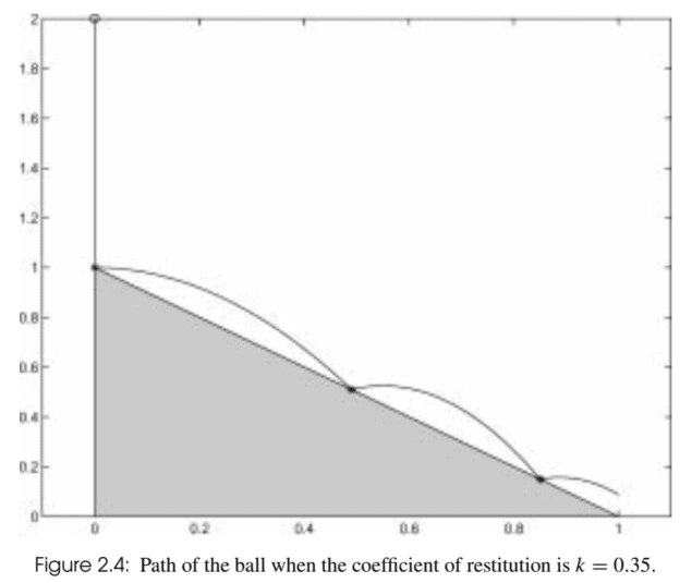
Along with the example programs of the text is a program $d f s . m$ that provides a modest capability for computing and plotting solutions of a scalar ODE, $y^{\prime}=f(t, y)$. Exercise $1.4$ discusses how to use this program, but only a few details are needed here. Solutions are plotted in a window that you specify by an array $[w L, w R, w B, w T]$. When you click on a point $\left(t_{0}, y_{0}\right)$, the program computes the solution $y(t)$ that has the initial value $y\left(t_{0}\right)=$ $y_{0}$ and plots it as long as $w L \leq t \leq w R$ and $w B \leq y \leq w T$. By calling ode 45 with interval $\left[t_{0}, w R\right]$, the program computes $y(t)$ from the initial point to the right edge of the plot window. It then calls the solver with the interval $\left[t_{0}, w L\right]$ to compute $y(t)$ from the initial point to the left edge. But what if the solution goes out the bottom or top of the plot window along the way? What we need is the capability of terminating the integration if there is a $t^{}$ where either $y\left(t^{}\right)=w B$ or $y\left(t^{*}\right)=w T$.
While approximating the solution of an IVP, we sometimes need to locate points $t^{}$ where certain event functions $$ g_{1}(t, y(t)), g_{2}(t, y(t)), \ldots, g_{k}(t, y(t)) $$ vanish. Determining these points is called event location. Sometimes we just want to know the solution, $y\left(t^{}\right)$, at the time, $t^{}$, of the event. On other occasions we need to terminate the integration at $t^{}$ and possibly start solving a new IVP with initial values and ODEs that depend on $t^{}$ and $y\left(t^{}\right)$. Sometimes it matters whether an event function is decreasing or increasing at the time of an event. In the dfs . m program, there are two event functions $(w B-y$ and $w T-y)$, both events are terminal, and we don’t care whether the event function is increasing or decreasing at an event. All the MATLAB IVP solvers have a powerful event location capability. Most continuous simulation languages and a few of the IVP solvers widely used in general scientific computing have some kind of capability of locating events. Event location can be ill-posed and some of the algorithms in use are crude. The difficulties of this task are often not appreciated, so one of the aims of this section is to instill some caution when using an event location capability. A deeper discussion of the issues can be found in Shampine, Gladwell, \& Brankin (1991) and Shampine \& Thompson (2000)
数学代写|matlab代写|ODEs Involving a Mass Matrix
Some solvers accept systems of ODEs written in forms more general than $y^{\prime}=f(t, y)$. In particular, the MATLAB IVP solvers accept problems of the form
$$
M(t, y) y^{\prime}=f(t, y)
$$
involving a mass matrix $M(t, y)$. If $M(t, y)$ is singular then this is a system of differential algebraic equations (DAEs). They are closely related to ODEs but differ in important ways. We do not pursue the solution of DAEs in this book beyond noting that the MATLAB codes for stiff ODEs can solve DAEs of index 1 arising in this way (Shampine, Reichelt, \& Kierzenka 1999). In Section 2.3.3 we discuss an approach to solving PDEs numerically that leads to systems of ODEs with a great many unknowns. Some of the schemes result in equations of the form (2.37). Example 2.3.11 provides more details about solving such problems.
In simplest use, the only difference when using a MATLAB IVP solver for a problem of the form (2.37) instead of a problem in standard form is that you must inform the solver about the presence of $M(t, y)$ by means of the option Mass. If the matrix is a constant then you should provide the matrix itself as the value of this option. The codes exploit constant mass matrices, so this is efficient as well as convenient. Suppose, for example, that you choose an explicit Runge-Kutta method. You provide the ODEs in the convenient form (2.37), but the solver actually applies the Runge-Kutta method to the ODEs
$$
y^{\prime}=F(t, y) \equiv M^{-1} f(t, y)
$$
which is in standard form. As the code initializes itself, it computes an $L U$ factorization of $M$. Whenever it needs to evaluate $F(t, y)$, it evaluates $f(t, y)$ and solves a linear system for $F$ using the stored factorization of $M$. For the solvers that proceed in this way, allowing a mass matrix is mainly a convenience for you. However, other solvers modify the methods themselves to include a mass matrix. Without going into the details, it should be no surprise that the iteration matrix for the BDFs is changed from $I-h \gamma J$ to $M-h \gamma J$. The iteration matrix must be factored in any case, so the extra cost of the more general form is unimportant. When the mass matrix is not constant, the modifications to the methods are more substantial. In this case, you must provide a (sub)function for evaluating the mass matrix and pass the name to the solver as the value of Mass.
数学代写|MATLAB代写|Large Systems and the Method of Lines
Now we take up issues that are important when solving an IVP for a large system of equations. The MATLAB PSE is not appropriate for the very large systems solved routinely in some areas of general scientific computing, but it is possible to solve conveniently systems that are quite large. The method of lines (MOL) is a way of approximating PDEs by ODEs. It leads naturally to large systems of equations that may be stiff. The MOL is a popular tool for solving PDEs, but we discuss it here mainly as a source of large systems of ODEs. MATLAB itself has an MOL code called pdepe that solves small systems of parabolic and elliptic PDEs in one space variable and time. Also, the MATLAB PDE Toolbox uses the MOL to solve PDEs in two space variables and time.
The idea of the MOL is to discretize all but one of the variables of a PDE so as to obtain a system of ODEs. This approach is called a semidiscretization. Typically the spatial variables are discretized and time is used as the continuous variable. There are several popular ways of discretizing the spatial variable. Two will be illustrated with an example taken from Trefethen (2000).
matlab代做
数学代写|MATLAB代写|EVENT LOCATION
与文本的示例程序一起是一个程序dFs.米为计算和绘制标量 ODE 的解提供适度的能力,是$d f s . m$ that provides a modest capability for computing and plotting solutions of a scalar ODE, $y^{\prime}=f(t, y)$. Exercise $1.4$ discusses how to use this program, but only a few details are needed here. Solutions are plotted in a window that you specify by an array $[w L, w R, w B, w T]$. When you click on a point $\left(t_{0}, y_{0}\right)$, the program computes the solution $y(t)$ that has the initial value $y\left(t_{0}\right)=$ $y_{0}$ and plots it as long as $w L \leq t \leq w R$ and $w B \leq y \leq w T$.. 通过间隔调用 ode 45[吨0,在R],程序计算是(吨)从初始点到绘图窗口的右边缘。然后它使用间隔调用求解器[吨0,在大号]计算是(吨)从初始点到左边缘。但是,如果解决方案沿途出现在绘图窗口的底部或顶部怎么办?如果存在$t^{}$ where either $y\left(t^{}\right)=w B$ or $y\left(t^{*}\right)=w T$.
在逼近 IVP 的解时,我们有时需要定位点 $t^{}$ where certain event functions $$ g_{1}(t, y(t)), g_{2}(t, y(t)), \ldots, g_{k}(t, y(t)) $$ vanish. Determining these points is called event location. Sometimes we just want to know the solution, $y\left(t^{}\right)$, at the time, $t^{}$, of the event. On other occasions we need to terminate the integration at $t^{}$ and possibly start solving a new IVP with initial values and ODEs that depend on $t^{}$ and $y\left(t^{}\right)$. Sometimes it matters whether an event function is decreasing or increasing at the time of an event. In the dfs . m program, there are two event functions $(w B-y$ and $w T-y)$,,这两个事件都是终端事件,我们不关心事件函数在事件中是增加还是减少。所有 MATLAB IVP 求解器都具有强大的事件定位功能。大多数连续模拟语言和一些广泛用于一般科学计算的 IVP 求解器都具有某种定位事件的能力。事件位置可能是不适定的,并且使用的一些算法很粗糙。此任务的困难通常不被理解,因此本节的目的之一是在使用事件定位功能时灌输一些谨慎。可以在 Shampine、Gladwell、\& Brankin 中找到对这些问题的更深入讨论1991和香平\&汤普森2000
数学代写|MATLAB代写|ODES INVOLVING A MASS MATRIX
一些求解器接受以比更一般的形式编写的 ODE 系统是′=F(吨,是). 特别是,MATLAB IVP 求解器接受以下形式的问题
米(吨,是)是′=F(吨,是)
涉及质量矩阵米(吨,是). 如果米(吨,是)是奇异的,那么这是一个微分代数方程组D一种和s. 它们与 ODE 密切相关,但在重要方面有所不同。除了注意到刚性 ODE 的 MATLAB 代码可以解决以这种方式产生的索引为 1 的 DAE 之外,我们在本书中不追求 DAE 的解决方案小号H一种米p一世n和,R和一世CH和l吨,&ķ一世和r和和nķ一种1999. 在第 2.3.3 节中,我们讨论了一种数值求解 PDE 的方法,该方法导致具有大量未知数的 ODE 系统。一些方案导致形式的方程2.37. 示例 2.3.11 提供了有关解决此类问题的更多详细信息。
在最简单的使用中,使用 MATLAB IVP 求解器解决以下形式的问题时的唯一区别2.37而不是标准形式的问题是您必须告知求解器存在米(吨,是)通过选项质量。如果矩阵是常数,那么您应该提供矩阵本身作为此选项的值。这些代码利用了恒定质量矩阵,因此既高效又方便。例如,假设您选择了一个显式的 Runge-Kutta 方法。您以方便的形式提供 ODE2.37,但求解器实际上将 Runge-Kutta 方法应用于 ODE
是′=F(吨,是)≡米−1F(吨,是)
这是标准形式。当代码初始化自身时,它计算一个大号在因式分解米. 每当它需要评估F(吨,是),它评估F(吨,是)并求解一个线性系统F使用存储的因式分解米. 对于以这种方式进行的求解器,允许使用质量矩阵主要是为了方便您。但是,其他求解器会修改方法本身以包含质量矩阵。在不深入细节的情况下,BDF 的迭代矩阵从一世−HCĴ到米−HCĴ. 在任何情况下都必须考虑迭代矩阵,因此更一般形式的额外成本并不重要。当质量矩阵不恒定时,对方法的修改更为实质性。在这种情况下,您必须提供s在b用于评估质量矩阵并将名称作为质量值传递给求解器的函数。
数学代写|MATLAB代写|LARGE SYSTEMS AND THE METHOD OF LINES
现在我们讨论在求解大型方程组的 IVP 时很重要的问题。MATLAB PSE 不适用于在一般科学计算的某些领域常规求解的超大型系统,但可以方便地求解相当大的系统。线的方法米这大号是一种通过 ODE 逼近 PDE 的方法。它自然会导致可能很僵硬的大型方程组。MOL 是求解 PDE 的流行工具,但我们在这里主要将其作为大型 ODE 系统的来源进行讨论。MATLAB 本身有一个称为 pdepe 的 MOL 代码,它可以在一个空间变量和时间内求解抛物线和椭圆 PDE 的小型系统。此外,MATLAB PDE Toolbox 使用 MOL 在两个空间变量和时间中求解 PDE。
MOL 的想法是离散 PDE 的一个变量以外的所有变量,以获得 ODE 系统。这种方法称为半离散化。通常,空间变量是离散的,时间用作连续变量。有几种流行的方法可以离散化空间变量。两个将用取自 Trefethen 的例子来说明2000.

数学代写|matlab代写 请认准UprivateTA™. UprivateTA™为您的留学生涯保驾护航。
微观经济学代写
微观经济学是主流经济学的一个分支,研究个人和企业在做出有关稀缺资源分配的决策时的行为以及这些个人和企业之间的相互作用。my-assignmentexpert™ 为您的留学生涯保驾护航 在数学Mathematics作业代写方面已经树立了自己的口碑, 保证靠谱, 高质且原创的数学Mathematics代写服务。我们的专家在图论代写Graph Theory代写方面经验极为丰富,各种图论代写Graph Theory相关的作业也就用不着 说。
线性代数代写
线性代数是数学的一个分支,涉及线性方程,如:线性图,如:以及它们在向量空间和通过矩阵的表示。线性代数是几乎所有数学领域的核心。
博弈论代写
现代博弈论始于约翰-冯-诺伊曼(John von Neumann)提出的两人零和博弈中的混合策略均衡的观点及其证明。冯-诺依曼的原始证明使用了关于连续映射到紧凑凸集的布劳威尔定点定理,这成为博弈论和数学经济学的标准方法。在他的论文之后,1944年,他与奥斯卡-莫根斯特恩(Oskar Morgenstern)共同撰写了《游戏和经济行为理论》一书,该书考虑了几个参与者的合作游戏。这本书的第二版提供了预期效用的公理理论,使数理统计学家和经济学家能够处理不确定性下的决策。
微积分代写
微积分,最初被称为无穷小微积分或 “无穷小的微积分”,是对连续变化的数学研究,就像几何学是对形状的研究,而代数是对算术运算的概括研究一样。
它有两个主要分支,微分和积分;微分涉及瞬时变化率和曲线的斜率,而积分涉及数量的累积,以及曲线下或曲线之间的面积。这两个分支通过微积分的基本定理相互联系,它们利用了无限序列和无限级数收敛到一个明确定义的极限的基本概念 。
计量经济学代写
什么是计量经济学?
计量经济学是统计学和数学模型的定量应用,使用数据来发展理论或测试经济学中的现有假设,并根据历史数据预测未来趋势。它对现实世界的数据进行统计试验,然后将结果与被测试的理论进行比较和对比。
根据你是对测试现有理论感兴趣,还是对利用现有数据在这些观察的基础上提出新的假设感兴趣,计量经济学可以细分为两大类:理论和应用。那些经常从事这种实践的人通常被称为计量经济学家。
Matlab代写
MATLAB 是一种用于技术计算的高性能语言。它将计算、可视化和编程集成在一个易于使用的环境中,其中问题和解决方案以熟悉的数学符号表示。典型用途包括:数学和计算算法开发建模、仿真和原型制作数据分析、探索和可视化科学和工程图形应用程序开发,包括图形用户界面构建MATLAB 是一个交互式系统,其基本数据元素是一个不需要维度的数组。这使您可以解决许多技术计算问题,尤其是那些具有矩阵和向量公式的问题,而只需用 C 或 Fortran 等标量非交互式语言编写程序所需的时间的一小部分。MATLAB 名称代表矩阵实验室。MATLAB 最初的编写目的是提供对由 LINPACK 和 EISPACK 项目开发的矩阵软件的轻松访问,这两个项目共同代表了矩阵计算软件的最新技术。MATLAB 经过多年的发展,得到了许多用户的投入。在大学环境中,它是数学、工程和科学入门和高级课程的标准教学工具。在工业领域,MATLAB 是高效研究、开发和分析的首选工具。MATLAB 具有一系列称为工具箱的特定于应用程序的解决方案。对于大多数 MATLAB 用户来说非常重要,工具箱允许您学习和应用专业技术。工具箱是 MATLAB 函数(M 文件)的综合集合,可扩展 MATLAB 环境以解决特定类别的问题。可用工具箱的领域包括信号处理、控制系统、神经网络、模糊逻辑、小波、仿真等。