
如果你也在 怎样代写高维数据分析High-Dimensional Data AnalysisI ETF5500这个学科遇到相关的难题,请随时右上角联系我们的24/7代写客服。高维数据分析High-Dimensional Data Analysis关注的是数据集,其中特征的数量与观察值的数量相当,甚至大于观察值的数量。这种类型的数据集带来了各种新的挑战,因为经典的理论和方法会以令人惊讶和意外的方式崩溃。
高维数据分析High-Dimensional Data Analysis伯克利的研究人员同时研究了在高维环境下出现的统计和计算挑战。在理论方面,他们从统计学、概率论和信息论中引入了一系列技术,包括经验过程理论、集中不等式,以及随机矩阵理论和自由概率。方法上的创新包括对矩阵频谱特性的新估计,草图和优化的随机化程序,以及在顺序设置中的决策算法。这项工作的动机和应用于各种科学和工程学科,包括计算生物学、天文学、推荐系统、金融时间序列和气候预测。
my-assignmentexpert™高维数据分析High-Dimensional Data Analysis代写,免费提交作业要求, 满意后付款,成绩80\%以下全额退款,安全省心无顾虑。专业硕 博写手团队,所有订单可靠准时,保证 100% 原创。my-assignmentexpert™, 最高质量的高维数据分析High-Dimensional Data Analysis作业代写,服务覆盖北美、欧洲、澳洲等 国家。 在代写价格方面,考虑到同学们的经济条件,在保障代写质量的前提下,我们为客户提供最合理的价格。 由于统计Statistics作业种类很多,同时其中的大部分作业在字数上都没有具体要求,因此高维数据分析High-Dimensional Data Analysis作业代写的价格不固定。通常在经济学专家查看完作业要求之后会给出报价。作业难度和截止日期对价格也有很大的影响。
想知道您作业确定的价格吗? 免费下单以相关学科的专家能了解具体的要求之后在1-3个小时就提出价格。专家的 报价比上列的价格能便宜好几倍。
my-assignmentexpert™ 为您的留学生涯保驾护航 在商科代写方面已经树立了自己的口碑, 保证靠谱, 高质且原创的商科代考服务。我们的专家在高维数据分析High-Dimensional Data Analysis代写方面经验极为丰富,各种高维数据分析High-Dimensional Data Analysis相关的作业也就用不着 说。
我们提供的高维数据分析High-Dimensional Data Analysis ETF5500及其相关学科的代写,服务范围广, 其中包括但不限于:
商科代写|高维数据分析代考High-Dimensional Data Analysis代考|Motivating examples
Conventional multiple testing procedures, such as the false discovery rate analyses (Benjamini and Hochberg 1995; Efron et al. 2001; Storey 2002; Genovese and Wasserman 2002; van der laan et al. 2004), implicitly assume that data are collected from repeated or identical experimental conditions, and hence the hypotheses are exchangeable. However, in many applications, data are known to be collected from heterogeneous sources and hypotheses intrinsically form into different groups.
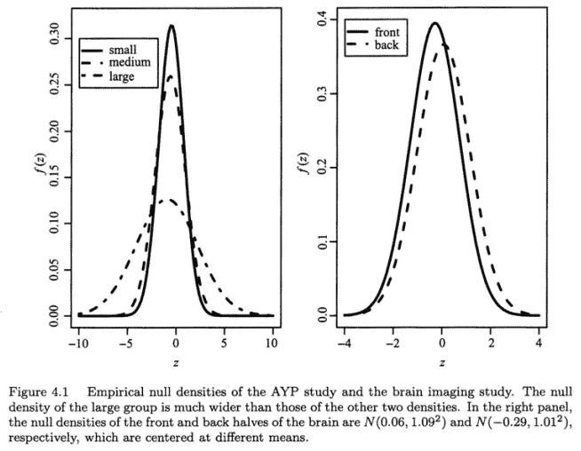
Consider the following two examples. The adequate yearly progress (AYP) study compares the academic performances of social-economically advantaged (SEA) versus social-economically disadvantaged (SED) students of California high schools (Rogosa 2003). Standard tests in mathematics were administered to 7867 schools and a $z$-value for comparing SEA and SED students was obtained for each school. The estimated null densities of the $z$-values for small, medium and large schools are plotted on the left panel of Figure 4.1. It is interesting to see that the null density of the large group is much wider than those of the other two densities. The differences in the null distributions have significant effects on the outcomes of a multiple testing procedure. Another example is the brain imaging study analyzed in Schwartzman et al. (2005). In this study, 6 dyslexic children and 6 normal children received diffusion tensor imaging brain scans on the same 15443 brain locations (voxels). A $z$-value (converted from a two-sample $t$-statistic) for comparing dyslexic versus normal children was obtained for each voxel. The right panel in Figure $4.1$ plots the estimated null densities of the $z$-values for the front and back halves of the brain. We can see that the null cases from two groups centered on different means, and the density of the back half is narrower. There are many other examples where the hypotheses are naturally grouped. For instance, in analysis of geographical survey data, individual locations are aggregated into several large clusters; and in meta-analysis of large biomedical studies, the data are collected from different clinical centers. An important common feature of these examples is that data are collected from heterogeneous sources and the hypotheses being considered are grouped and no longer exchangeable. We shall see that incorporating the grouping information is important for optimal simultaneous inference with samples collected from different groups.
商科代写|高维数据分析代考High-Dimensional Data Analysis代考|The multiple-group model
The multiple-group random mixture model (Efron 2008a; see Figure 4.2) extends the previous random mixture model (3.1) (for a single group) to cover the situation where the $m$ cases can be divided into $K$ groups. It is assumed that within each group, the random mixture model (3.1) holds separately.
Let $\boldsymbol{g}=\left(g_{1}, \ldots, g_{K}\right)$ be a multinomial variable with probabilities $\left{\pi_{1}, \ldots, \pi_{K}\right}$, where $g_{i}=k$ indicates that case $i$ belongs to group $k$. We assume that prior to analysis, the group labels $g$ have been determined by external information derived from other data or a priori knowledge. Let $\boldsymbol{\theta}=\left(\theta_{1}, \ldots, \theta_{m}\right)$ be Bernoulli variables, where $\theta_{i}=1$ indicates that case $i$ is a non-null and $\theta_{i}=0$ otherwise. Given $\boldsymbol{g}$, $\boldsymbol{\theta}$ can be grouped as $\boldsymbol{\theta}=\left(\boldsymbol{\theta}{1}, \ldots, \boldsymbol{\theta}{K}\right)=\left{\left(\theta_{k 1}, \ldots, \theta_{k m_{k}}\right): k=1, \ldots, K\right}$, where $m_{k}$ is the number of hypotheses in group $k$. Different from $g, \theta$ are unknown and need to be inferred from observations $\boldsymbol{x}$. Let $\theta_{k i}, i=1, \ldots, m_{k}$, be independent Bernoulli $\left(p_{k}\right)$ variables and $\boldsymbol{X}=\left(X_{k i}\right)$ be generated conditional on $\boldsymbol{\theta}$ :
$$
X_{k i} \mid \theta_{k i} \sim\left(1-\theta_{k i}\right) F_{k 0}+\theta_{k i} F_{k 1}, i=1, \ldots, m_{k}, k=1, \ldots, K
$$
Hence within group $k$, the $X_{k i}$ ‘s, $i=1, \ldots, m_{k}$, are i.i.d. observations with mixture distribution $F_{k}=\left(1-p_{k}\right) F_{k 0}+p_{k} F_{k 1}$. Denote by $f_{k}$ the mixture density of group $k$, the null and non-null densities by $f_{k 0}$ and $f_{k 1}$, respectively. Then $f_{k}=$ $\left(1-p_{k}\right) f_{k 0}+p_{k} f_{k 1}$
高维数据分析代考
商科代写|高维数据分析代㛈HIGH-DIMENSIONAL DATA ANALYSIS代考|MOTIVATING EXAMPLES
传统的多重测诖程序,例如错误发现率分析
BenjaminiandHochberg $1995 ;$ E fronetal. 2001; Storey 2002 ; Genoveseand Wasserman $2002 ;$ vanderlaanetal. 2004,隐含地假设数据是从重复或相同的实 验条件中收集的,因此假设是可交换的。然而,在许多应用中,已知数据是从㫒构来源收集的,并且假设本质上形成不同的组。
考虑以下两个示例。充足的年度进展 $A Y P$ 研究比较了具有社会经济优势的学生的学业成绩 $S E A$ 与社会经济弱势群体相比 SED加州高中学生Rogosa2003. 对 7867 所 学校和一所学校进行了数学标准测试 $z$-为每所学校获得了用于比较 SEA 和 SED 学生的值。估计的零密度 $z$ – 小型、中型和大型学校的值绘制在图 4.1 的左侧面板上。有趗 的是,大群的函密度比其他两个密度要宽得多。零分布的差异对多重测试过程的结果有显着影响。另一个例子是 Schwartzman 等人分析的脑成像研究。2005. 在这项㓈 究,6名阅读障碍儿童和 6 名正常儿童在相同的 $15443 \mathrm{~ 个 大 脑 伩 置 接 愛}$ 为每个体素获得了用于比较阅读障碍与正常儿童的比较。图中右侧面板 $4.1$ 绘制估计的零密度 $z$-大脑前半部分和后半部分的值。我们可以看到,两组的空安例集中在不 同的均值上,后半部分的密度更害。还有很多其他的例子,假设是自然分组的。例如,在分析地理调查数据时,将各个位置聚合成几个大集群; 在大型生物医学研究的 荟萃分析中,数据是从不同的临床中心收集的。这些示例的一个重要共同特征是数据是从异构来源收集的,并且正在考虑的假设被分组并且不再可交换。我们将看到, 合并分组信息对于从不同组收集的样本进行最佳同时推理很重要。
商科代写|高维数据分析代考HIGH-DIMENSIONAL DATA ANALYSIS代考|THE MULTIPLE-GROUP MODEL
多组随机混合模型Efron $2008 a ;$ seeFigure $4.2$ 扩展了之前的随机混合模型3.1 forasinglegroup嘌盖的情况m安例可以分为 $K$ 团体。假设在每组内,随机混合模型 $3.1$ 分开持有。 让 $g=\left(g_{1}, \ldots, g_{K}\right) \mathrm{~ 是 具 有 概 率 的 茤 项 变 量 ~ \ l e f t { 1 p i _ { 1 ] ,}$ 知识派生的外部信息确定。让 $\theta=\left(\theta_{1}, \ldots, \theta_{m}\right)$ 是伯妓利变量,其中 $\theta_{i}=1$ 表示这种情况 $i$ 是非空的并且 $\theta_{i}=0$ 否则。给定 $g, \theta$ 可以归关为 数量 $k$. 不同于 $g, \theta$ 末知,需要从观察中推断 $\boldsymbol{x}$. 让 $\theta_{k i}, i=1, \ldots, m_{k}$, 独立伯努利 $\left(p_{k}\right)$ 变量和 $\boldsymbol{X}=\left(X_{k i}\right)$ 生成条件 $\theta$ :
$$
X_{k i} \mid \theta_{k i} \sim\left(1-\theta_{k i}\right) F_{k 0}+\theta_{k i} F_{k 1}, i=1, \ldots, m_{k}, k=1, \ldots, K
$$
因此在组内 $k$ ,这 $X_{k i}$ 的, $i=1, \ldots, m_{k}$, 是具有混合分布的独立同分布观察 $F_{k}=\left(1-p_{k}\right) F_{k 0}+p_{k} F_{k 1}$. 表示为 $f_{k}$ 群的混合密度 $k$ ,零和非零密度由 $f_{k 0}$ 和 $f_{k 1}$ ,分 别。然后 $f_{k}=\left(1-p_{k}\right) f_{k 0}+p_{k} f_{k 1}$

澳洲代考|高维数据分析代考HIGH-DIMENSIONAL DATA ANALYSIS代考 请认准UprivateTA™. UprivateTA™为您的留学生涯保驾护航。
微观经济学代写
微观经济学是主流经济学的一个分支,研究个人和企业在做出有关稀缺资源分配的决策时的行为以及这些个人和企业之间的相互作用。my-assignmentexpert™ 为您的留学生涯保驾护航 在数学Mathematics作业代写方面已经树立了自己的口碑, 保证靠谱, 高质且原创的数学Mathematics代写服务。我们的专家在图论代写Graph Theory代写方面经验极为丰富,各种图论代写Graph Theory相关的作业也就用不着 说。
线性代数代写
线性代数是数学的一个分支,涉及线性方程,如:线性图,如:以及它们在向量空间和通过矩阵的表示。线性代数是几乎所有数学领域的核心。
博弈论代写
现代博弈论始于约翰-冯-诺伊曼(John von Neumann)提出的两人零和博弈中的混合策略均衡的观点及其证明。冯-诺依曼的原始证明使用了关于连续映射到紧凑凸集的布劳威尔定点定理,这成为博弈论和数学经济学的标准方法。在他的论文之后,1944年,他与奥斯卡-莫根斯特恩(Oskar Morgenstern)共同撰写了《游戏和经济行为理论》一书,该书考虑了几个参与者的合作游戏。这本书的第二版提供了预期效用的公理理论,使数理统计学家和经济学家能够处理不确定性下的决策。
微积分代写
微积分,最初被称为无穷小微积分或 “无穷小的微积分”,是对连续变化的数学研究,就像几何学是对形状的研究,而代数是对算术运算的概括研究一样。
它有两个主要分支,微分和积分;微分涉及瞬时变化率和曲线的斜率,而积分涉及数量的累积,以及曲线下或曲线之间的面积。这两个分支通过微积分的基本定理相互联系,它们利用了无限序列和无限级数收敛到一个明确定义的极限的基本概念 。
计量经济学代写
什么是计量经济学?
计量经济学是统计学和数学模型的定量应用,使用数据来发展理论或测试经济学中的现有假设,并根据历史数据预测未来趋势。它对现实世界的数据进行统计试验,然后将结果与被测试的理论进行比较和对比。
根据你是对测试现有理论感兴趣,还是对利用现有数据在这些观察的基础上提出新的假设感兴趣,计量经济学可以细分为两大类:理论和应用。那些经常从事这种实践的人通常被称为计量经济学家。
Matlab代写
MATLAB 是一种用于技术计算的高性能语言。它将计算、可视化和编程集成在一个易于使用的环境中,其中问题和解决方案以熟悉的数学符号表示。典型用途包括:数学和计算算法开发建模、仿真和原型制作数据分析、探索和可视化科学和工程图形应用程序开发,包括图形用户界面构建MATLAB 是一个交互式系统,其基本数据元素是一个不需要维度的数组。这使您可以解决许多技术计算问题,尤其是那些具有矩阵和向量公式的问题,而只需用 C 或 Fortran 等标量非交互式语言编写程序所需的时间的一小部分。MATLAB 名称代表矩阵实验室。MATLAB 最初的编写目的是提供对由 LINPACK 和 EISPACK 项目开发的矩阵软件的轻松访问,这两个项目共同代表了矩阵计算软件的最新技术。MATLAB 经过多年的发展,得到了许多用户的投入。在大学环境中,它是数学、工程和科学入门和高级课程的标准教学工具。在工业领域,MATLAB 是高效研究、开发和分析的首选工具。MATLAB 具有一系列称为工具箱的特定于应用程序的解决方案。对于大多数 MATLAB 用户来说非常重要,工具箱允许您学习和应用专业技术。工具箱是 MATLAB 函数(M 文件)的综合集合,可扩展 MATLAB 环境以解决特定类别的问题。可用工具箱的领域包括信号处理、控制系统、神经网络、模糊逻辑、小波、仿真等。