如果你也在 怎样代写有限元Finite Element ENGR7961个学科遇到相关的难题,请随时右上角联系我们的24/7代写客服。有限元Finite Element Method是一种流行的方法,用于数值解决工程和数学建模中出现的微分方程。典型的问题领域包括结构分析、传热、流体流动、质量运输和电磁势等传统领域。
有限元Finite Element Method是一种通用的数值方法,用于解决两个或三个空间变量的偏微分方程(即一些边界值问题)。为了解决一个问题,有限元将一个大系统细分为更小、更简单的部分,称为有限元。这是通过在空间维度上的特定空间离散化来实现的,它是通过构建对象的网格来实现的:用于求解的数值域,它有有限数量的点。边界值问题的有限元法表述最终导致一个代数方程组。该方法在域上对未知函数进行逼近。然后将模拟这些有限元的简单方程组合成一个更大的方程系统,以模拟整个问题。然后,有限元通过变化微积分使相关的误差函数最小化来逼近一个解决方案。
有限元Finite Element Method代写,免费提交作业要求, 满意后付款,成绩80\%以下全额退款,安全省心无顾虑。专业硕 博写手团队,所有订单可靠准时,保证 100% 原创。 最高质量的有限元Finite Element Method作业代写,服务覆盖北美、欧洲、澳洲等 国家。 在代写价格方面,考虑到同学们的经济条件,在保障代写质量的前提下,我们为客户提供最合理的价格。 由于作业种类很多,同时其中的大部分作业在字数上都没有具体要求,因此有限元Finite Element Method作业代写的价格不固定。通常在专家查看完作业要求之后会给出报价。作业难度和截止日期对价格也有很大的影响。
同学们在留学期间,都对各式各样的作业考试很是头疼,如果你无从下手,不如考虑my-assignmentexpert™!
my-assignmentexpert™提供最专业的一站式服务:Essay代写,Dissertation代写,Assignment代写,Paper代写,Proposal代写,Proposal代写,Literature Review代写,Online Course,Exam代考等等。my-assignmentexpert™专注为留学生提供Essay代写服务,拥有各个专业的博硕教师团队帮您代写,免费修改及辅导,保证成果完成的效率和质量。同时有多家检测平台帐号,包括Turnitin高级账户,检测论文不会留痕,写好后检测修改,放心可靠,经得起任何考验!
想知道您作业确定的价格吗? 免费下单以相关学科的专家能了解具体的要求之后在1-3个小时就提出价格。专家的 报价比上列的价格能便宜好几倍。
我们在数学Mathematics代写方面已经树立了自己的口碑, 保证靠谱, 高质且原创的数学Mathematics代写服务。我们的专家在有限元Finite Element Method代写方面经验极为丰富,各种有限元Finite Element Method相关的作业也就用不着 说。

数学代写|有限元代写Finite Element Method代考|Boundary Conditions
There are two types of boundary conditions: displacement (essential) and force (natural) boundary conditions. The displacement boundary condition can be simply written as
$$
u=\bar{u} \quad \text { and/or } \quad v=\bar{v} \quad \text { and/or } \quad w=\bar{w}
$$
on displacement boundaries. The bar stands for the prescribed value for the displacement component. For most of the actual simulations, the displacement is used to describe the support or constraints on the solid, and hence the prescribed displacement values are often zero. In such cases, the boundary condition is termed as a homogenous boundary condition. Otherwise, they are inhomogeneous boundary conditions.
The force boundary condition are often written as
$$
\mathbf{n} \sigma=\overline{\mathbf{t}}
$$
on force boundaries, where $\mathbf{n}$ is given by
$$
\mathbf{n}=\left[\begin{array}{cccccc}
n_x & 0 & 0 & 0 & n_z & n_y \
0 & n_y & 0 & n_z & 0 & n_x \
0 & 0 & n_z & n_y & n_x & 0
\end{array}\right]
$$
in which $n_i(i=x, y, z)$ are cosines of the outwards normal on the boundary. The bar stands for the prescribed value for the force component. A force boundary condition can also be both homogenous and inhomogeneous. If the condition is homogeneous, it implies that the boundary is a free surface.
The reader may naturally ask why the displacement boundary condition is called an essential boundary condition and the force boundary condition is called a natural boundary conditions. The terms ‘essential’ and ‘natural’ come from the use of the so-called weak form formulation (such as the weighted residual method) for deriving system equations. In such a formulation process, the displacement condition has to be satisfied first before derivation starts, or the process will fail. Therefore, the displacement condition is essential. As long as the essential (displacement) condition is satisfied, the process will lead to the equilibrium equations as well as the force boundary conditions. This means that the force boundary condition is naturally derived from the process, and it is therefore called the natural boundary condition. Since the terms essential and natural boundary do not describe used for problems other than in mechanics.
Equations obtained in this section are applicable to 3D solids. The objective of most analysts is to solve the equilibrium equations and obtain the solution of the field variable, which in this case is the displacement. Theoretically, these equations can be applied to all other types of structures such as trusses, beams, plates and shells, because physically they are all 3D in nature. However, treating all the structural components as 3D solids makes computation very expensive, and sometimes practically impossible. Therefore, theories for taking geometrical advantage of different types of solids and structural components have been developed. Application of these theories in a proper manner can reduce the analytical and computational effort drastically. A brief description of these theories is given in the following sections.
数学代写|有限元代写Finite Element Method代考|Stress and Strain
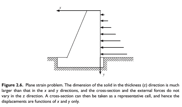
Three-dimensional problems can be drastically simplified if they can be treated as a twodimensional (2D) solid. For representation as a 2D solid, we basically try to remove one coordinate (usually the $z$-axis), and hence assume that all the dependent variables are independent of the $z$-axis, and all the external loads are independent of the $z$ coordinate, and applied only in the $x-y$ plane. Therefore, we are left with a system with only two coordinates, the $x$ and the $y$ coordinates. There are primarily two types of 2D solids. One is a plane stress solid, and another is a plane strain solid. Plane stress solids are solids whose thickness in the $z$ direction is very small compared with dimensions in the $x$ and $y$ directions. External forces are applied only in the $x-y$ plane, and stresses in the $z$ direction $\left(\sigma_{z z}, \sigma_{x z}, \sigma_{y z}\right)$ are all zero, as shown in Figure 2.5. Plane strain solids are those solids whose thickness in the $z$ direction is very large compared with the dimensions in the $x$ and $y$ directions. External forces are applied evenly along the $z$ axis, and the movement in the $z$ direction at any point is constrained. The strain components in the $z$ direction $\left(\varepsilon_{z z}, \varepsilon_{x z}, \varepsilon_{y z}\right)$ are, therefore, all zero, as shown in Figure 2.6.
Note that for the plane stress problems, the strains $\varepsilon_{x z}$ and $\varepsilon_{y z}$ are zero, but $\varepsilon_{z z}$ will not be zero. It can be recovered easily using Eq.(2.9) after the in-plan stresses are obtained.
有限元代写
数学代写|有限元代写有限元法代考|边界条件
有两种边界条件:位移(必要的)和力(自然的)边界条件。位移边界条件可以简单地写成位移边界上
$$
u=\bar{u} \quad \text { and/or } \quad v=\bar{v} \quad \text { and/or } \quad w=\bar{w}
$$
。横条表示位移分量的规定值。对于大多数实际模拟,位移被用来描述固体上的支撑或约束,因此规定的位移值通常为零。在这种情况下,边界条件称为齐次边界条件。否则为非齐次边界条件。
力边界条件通常写为在力边界上
$$
\mathbf{n} \sigma=\overline{\mathbf{t}}
$$
,其中$\mathbf{n}$由
$$
\mathbf{n}=\left[\begin{array}{cccccc}
n_x & 0 & 0 & 0 & n_z & n_y \
0 & n_y & 0 & n_z & 0 & n_x \
0 & 0 & n_z & n_y & n_x & 0
\end{array}\right]
$$
给出,其中$n_i(i=x, y, z)$是边界上向外法线的余弦。横条表示力分量的规定值。力的边界条件也可以是均匀的和非均匀的。如果条件是齐次的,它意味着边界是一个自由曲面
读者可能会自然地问,为什么位移边界条件被称为本质边界条件,力边界条件被称为自然边界条件?术语“本质”和“自然”来自于使用所谓的弱形式公式(如加权残差法)来推导系统方程。在这样的推导过程中,在推导开始之前必须首先满足位移条件,否则过程将失败。因此,位移条件是必要的。只要满足基本(位移)条件,这个过程就会得到平衡方程和力边界条件。这意味着力边界条件是自然地从过程中推导出来的,因此称为自然边界条件。由于“本质边界”和“自然边界”这两个术语不能用来描述力学以外的问题
本节得到的方程适用于三维固体。大多数分析人员的目标是求解平衡方程并得到场变量的解,在这种情况下,场变量就是位移。理论上,这些方程可以应用于所有其他类型的结构,如桁架、梁、板和壳,因为在物理上它们都是3D的本质。然而,将所有的结构组件都作为3D固体处理会使计算非常昂贵,有时实际上是不可能的。因此,利用不同类型的固体和结构组件的几何优势的理论已经发展起来。适当地应用这些理论可以大大减少分析和计算的工作量。下面几节将简要介绍这些理论
数学代写|有限元代写有限元法代考|应力与应变
如果三维问题可以被当作二维(2D)固体来处理,它们就可以大大简化。对于二维实体的表示,我们基本上尝试删除一个坐标(通常是$z$ -轴),因此假设所有因变量都独立于$z$ -轴,所有外部负载都独立于$z$坐标,并且只应用于$x-y$平面。因此,我们得到的系统只有两个坐标,$x$和$y$坐标。二维固体主要有两种类型。一个是平面应力实心,另一个是平面应变实心。平面应力固体是指$z$方向的厚度与$x$和$y$方向的尺寸相比非常小的固体。仅在$x-y$平面施加外力,$z$方向$\left(\sigma_{z z}, \sigma_{x z}, \sigma_{y z}\right)$的应力均为零,如图2.5所示。平面应变固形物是指$z$方向的厚度比$x$和$y$方向尺寸大的固形物。沿$z$轴均匀施加外力,在$z$方向上的任何一点的运动都受到约束。因此,$z$方向$\left(\varepsilon_{z z}, \varepsilon_{x z}, \varepsilon_{y z}\right)$上的应变分量均为零,如图2.6所示。
注意,对于平面应力问题,应变$\varepsilon_{x z}$和$\varepsilon_{y z}$为零,但$\varepsilon_{z z}$不为零。在获得平面内应力后,可以很容易地使用式(2.9)进行恢复

数学代写|有限元代写Finite Element Method代考 请认准UprivateTA™. UprivateTA™为您的留学生涯保驾护航。
微观经济学代写
微观经济学是主流经济学的一个分支,研究个人和企业在做出有关稀缺资源分配的决策时的行为以及这些个人和企业之间的相互作用。my-assignmentexpert™ 为您的留学生涯保驾护航 在数学Mathematics作业代写方面已经树立了自己的口碑, 保证靠谱, 高质且原创的数学Mathematics代写服务。我们的专家在图论代写Graph Theory代写方面经验极为丰富,各种图论代写Graph Theory相关的作业也就用不着 说。
线性代数代写
线性代数是数学的一个分支,涉及线性方程,如:线性图,如:以及它们在向量空间和通过矩阵的表示。线性代数是几乎所有数学领域的核心。
博弈论代写
现代博弈论始于约翰-冯-诺伊曼(John von Neumann)提出的两人零和博弈中的混合策略均衡的观点及其证明。冯-诺依曼的原始证明使用了关于连续映射到紧凑凸集的布劳威尔定点定理,这成为博弈论和数学经济学的标准方法。在他的论文之后,1944年,他与奥斯卡-莫根斯特恩(Oskar Morgenstern)共同撰写了《游戏和经济行为理论》一书,该书考虑了几个参与者的合作游戏。这本书的第二版提供了预期效用的公理理论,使数理统计学家和经济学家能够处理不确定性下的决策。
微积分代写
微积分,最初被称为无穷小微积分或 “无穷小的微积分”,是对连续变化的数学研究,就像几何学是对形状的研究,而代数是对算术运算的概括研究一样。
它有两个主要分支,微分和积分;微分涉及瞬时变化率和曲线的斜率,而积分涉及数量的累积,以及曲线下或曲线之间的面积。这两个分支通过微积分的基本定理相互联系,它们利用了无限序列和无限级数收敛到一个明确定义的极限的基本概念 。
计量经济学代写
什么是计量经济学?
计量经济学是统计学和数学模型的定量应用,使用数据来发展理论或测试经济学中的现有假设,并根据历史数据预测未来趋势。它对现实世界的数据进行统计试验,然后将结果与被测试的理论进行比较和对比。
根据你是对测试现有理论感兴趣,还是对利用现有数据在这些观察的基础上提出新的假设感兴趣,计量经济学可以细分为两大类:理论和应用。那些经常从事这种实践的人通常被称为计量经济学家。
Matlab代写
MATLAB 是一种用于技术计算的高性能语言。它将计算、可视化和编程集成在一个易于使用的环境中,其中问题和解决方案以熟悉的数学符号表示。典型用途包括:数学和计算算法开发建模、仿真和原型制作数据分析、探索和可视化科学和工程图形应用程序开发,包括图形用户界面构建MATLAB 是一个交互式系统,其基本数据元素是一个不需要维度的数组。这使您可以解决许多技术计算问题,尤其是那些具有矩阵和向量公式的问题,而只需用 C 或 Fortran 等标量非交互式语言编写程序所需的时间的一小部分。MATLAB 名称代表矩阵实验室。MATLAB 最初的编写目的是提供对由 LINPACK 和 EISPACK 项目开发的矩阵软件的轻松访问,这两个项目共同代表了矩阵计算软件的最新技术。MATLAB 经过多年的发展,得到了许多用户的投入。在大学环境中,它是数学、工程和科学入门和高级课程的标准教学工具。在工业领域,MATLAB 是高效研究、开发和分析的首选工具。MATLAB 具有一系列称为工具箱的特定于应用程序的解决方案。对于大多数 MATLAB 用户来说非常重要,工具箱允许您学习和应用专业技术。工具箱是 MATLAB 函数(M 文件)的综合集合,可扩展 MATLAB 环境以解决特定类别的问题。可用工具箱的领域包括信号处理、控制系统、神经网络、模糊逻辑、小波、仿真等。