
如果你也在 怎样代写计算机视觉Computer Vision EECS498-007这个学科遇到相关的难题,请随时右上角联系我们的24/7代写客服。计算机视觉Computer Vision是人工智能(AI)的一个领域,使计算机和系统能够从数字图像、视频和其他视觉输入中获得有意义的信息–并根据这些信息采取行动或提出建议。如果说人工智能使计算机能够思考,那么计算机视觉则使它们能够看到、观察和理解。
计算机视觉Computer Vision任务包括获取、处理、分析和理解数字图像的方法,以及从现实世界中提取高维数据以产生数字或符号信息,例如以决策的形式。这里的理解意味着将视觉图像(视网膜的输入)转化为对思维过程有意义的世界描述,并能引起适当的行动。这种图像理解可以被看作是利用借助几何学、物理学、统计学和学习理论构建的模型将符号信息从图像数据中分离出来的过程。
计算机视觉Computer Vision代写,免费提交作业要求, 满意后付款,成绩80\%以下全额退款,安全省心无顾虑。专业硕 博写手团队,所有订单可靠准时,保证 100% 原创。 最高质量的计算机视觉Computer Vision作业代写,服务覆盖北美、欧洲、澳洲等 国家。 在代写价格方面,考虑到同学们的经济条件,在保障代写质量的前提下,我们为客户提供最合理的价格。 由于作业种类很多,同时其中的大部分作业在字数上都没有具体要求,因此计算机视觉Computer Vision作业代写的价格不固定。通常在专家查看完作业要求之后会给出报价。作业难度和截止日期对价格也有很大的影响。
同学们在留学期间,都对各式各样的作业考试很是头疼,如果你无从下手,不如考虑my-assignmentexpert™!
my-assignmentexpert™提供最专业的一站式服务:Essay代写,Dissertation代写,Assignment代写,Paper代写,Proposal代写,Proposal代写,Literature Review代写,Online Course,Exam代考等等。my-assignmentexpert™专注为留学生提供Essay代写服务,拥有各个专业的博硕教师团队帮您代写,免费修改及辅导,保证成果完成的效率和质量。同时有多家检测平台帐号,包括Turnitin高级账户,检测论文不会留痕,写好后检测修改,放心可靠,经得起任何考验!
想知道您作业确定的价格吗? 免费下单以相关学科的专家能了解具体的要求之后在1-3个小时就提出价格。专家的 报价比上列的价格能便宜好几倍。
我们在计算机Quantum computer代写方面已经树立了自己的口碑, 保证靠谱, 高质且原创的计算机Quantum computer代写服务。我们的专家在计算机视觉Computer Vision代写方面经验极为丰富,各种计算机视觉Computer Vision相关的作业也就用不着 说。
计算机代写|计算机视觉代写Computer Vision代考|Iterative Multidimensional Optimization: General Proceeding
The techniques presented in this chapter are universally applicable, because they:
Directly operate on the energy function $f(x)$.
Do not rely on a special structure of $f(x)$.
The broadest possible applicability can be achieved if only information about the values of $f(x)$ themselves is required.
The other side of the coin is that these methods are usually rather slow. Therefore, some of the methods of the following sections additionally utilize knowledge about the first- and second-order derivatives $f^{\prime}(x)$ and $f^{\prime \prime}(x)$. This restricts their applicability a bit in exchange for an acceleration of the solution calculation. As was already stated earlier, it usually is best to make use of as much specific knowledge about the optimization problem at hand as possible. The usage of this knowledge will typically lead to faster algorithms.
Furthermore, as the methods of this chapter typically perform a local search, there is no guarantee that the global optimum is found. In order to avoid to get stuck in a local minimum, a reasonably good first estimate $x_0$ of the minimal position $x^*$ is required for those methods.
The general proceeding of most of the methods presented in this chapter is a two-stage iterative approach. Usually, the function $f(\mathbf{x})$ is vector valued, i.e., $\mathbf{x}$ consists of multiple ( say $N$ ) elements. Hence, the optimization procedure has to find $N$ values simultaneously. Starting at an initial solution $\mathbf{x}^k$, this can be done by an iterated application of the following two steps:
Calculation of a so-called search direction $\mathbf{s}^k$ along which the minimal position is to be searched.
Update the solution by finding a $\mathbf{x}^{k+1}$ which reduces $f\left(\mathbf{x}^{k+1}\right)$ (compared to $f\left(\mathbf{x}^k\right)$ ) by performing a one-dimensional search along the direction $\mathbf{s}^k$. Because $\mathbf{s}^k$ remains fixed during one iteration, this step is also called a line search. Mathematically, this can be written as
$$
\mathbf{x}^{k+1}=\mathbf{x}^k+\alpha^k \cdot \mathbf{s}^k
$$
where, in the most simple case, $\alpha^k$ is a fixed step size or – more sophisticated – is estimated during the one-dimensional search such that $\mathbf{x}^{k+1}$ minimizes the objective function along the search direction $\mathbf{s}^k$. The repeated procedure stops either if convergence is achieved, i.e., $f\left(\mathbf{x}^{k+1}\right)$ is sufficiently close to $f\left(\mathbf{x}^k\right)$ and hence we assume that no more progress is possible, or if the number of iterations exceeds an upper threshold $K_{\max }$. This iterative process is visualized in Fig. $2.3$ with the help of a rather simple example objective function.
计算机代写|计算机视觉代写Computer Vision代考|One-Dimensional Optimization Along a Search Direction
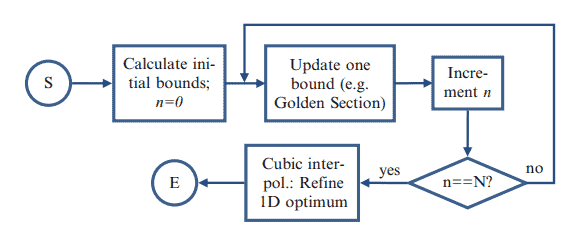
In this section, step two of the general iterative procedure is discussed in more detail. The outline of the proceeding of this step is to first bound the solution and subsequently iteratively narrow down the bounds until it is possible to interpolate the solution with good accuracy. In more detail, the one-dimensional optimization comprises the following steps (see also flowchart of Fig. 2.4):
- Determine upper and lower bounds $\mathbf{x}_u^k=\mathbf{x}^k+\alpha_u^0 \cdot \mathbf{s}^k$ and $\mathbf{x}_l^k=\mathbf{x}^k+\alpha_l^0 \cdot \mathbf{s}^k$ which bound the current solution $\mathbf{x}^k$ ( $\alpha_u^0$ and $\alpha_l^0$ have opposite signs).
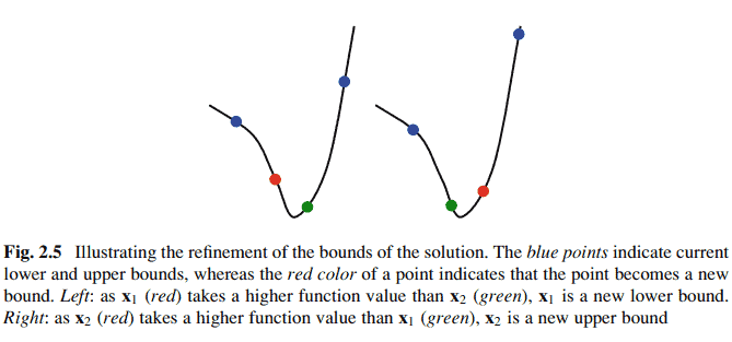
- Recalculate the upper and lower bounds $\mathbf{x}_u^i$ and $\mathbf{x}_l^i$ in an iterative scheme, i.e., decrease the distance between $\mathbf{x}_u^i$ and $\mathbf{x}_l^i$ as the iteration proceeds. Please note that, for a better understanding, the superscript $\boldsymbol{k}$ indicating the index of the multidimensional iteration is dropped and replaced by the index $i$ of the current one-dimensional iteration. One possibility to update the bounds is the so-called golden section method, which will be presented below. As the distance between the bounds is reduced by a fixed fraction at each iteration there, we can set the number of iterations necessary to a fixed value $N$.
- Refine the solution by applying a polynomial interpolation to the data found in step 2, where the refined bounds $\mathbf{x}_u^i$ and $\mathbf{x}_l^i$ as well as two intermediate points were found (see below). Hence, we have four data points and can perform a cubic interpolation based on these four points.
计算机视觉代写
计算机代写计算机视觉代写COMPUTER VISION代 考|ITERATIVE MULTIDIMENSIONAL OPTIMIZATION: GENERAL PROCEEDING
本章介绍的技术普遍适用,因为它们:
直接对能量函数进行运算 $f(x)$.
不要依赖特殊的结构 $f(x)$.
如果只有关于价值的信息,就可以实现最广泛的适用 $f(x)$ 自己是必需的。
硬币的另一面是这些方法通常相当慢。因此,以下部分的一些方法额外利用了关于一阶和二阶导数的知识 $f^{\prime}(x)$ 和 $f^{\prime \prime}(x)$. 这限制了它们的适用性,以换取解决方案 计算的加速。如前所述,通常最好层可能岁地利用手头优化问题的具体知识。这些知识的使用通常会导致更快的算法。 的。 开始 $\mathbf{x}^k ,$ 这可以通过以下两个步䇯的迭代应用来完成:
计算所佣的搜索方向 $\mathrm{s}^k$ 沿其搜索最小位置。
. Because $\mid$ mathbf []$^{\wedge} \mathrm{kremains}$ fixedduringoneiteration, thisstepisalsocalledalinesearch. Mathematically, thiscanbewrittenas $\mathrm{x}^{k+1}=\mathrm{x}^k+\alpha^k \cdot \mathrm{s}^k$
where, inthemostsimplecase, $\backslash$ alpha^kisafixedstepsizeor-moresophisticated-isestimatedduringtheone-dimensionalsearchsuchthat
andhenceweassumethatnomoreprogressispossible, orifthenumberofiterationsexceedsanupperthresholdK_{\最大}
Thisiterativeprocessisvisualizedin Fig. $2.3 \$$ 借助一个相当简单的示例目标函数。
计算机代写计算机视觉代写COMPUTER VISION代考|ONEDIMENSIONAL OPTIMIZATION ALONG A SEARCH DIRECTION
在本节中,将更详细地讨论一般迭代过程的第二步。此步癹的概要是首先限制解,然后迭代地缩小边界,直到可以以良好的精度对解进行揷值。更详细地说,一维 优化包括以下步骙 seealsoflowchartofFig. 2.4:
- 确定上限和下限 $\mathbf{x}_u^k=\mathbf{x}^k+\alpha_u^0 \cdot \mathbf{s}^k$ 和 $\mathbf{x}_l^k=\mathbf{x}^k+\alpha_l^0 \cdot \mathbf{s}^k$ 这限制了当前的解决方客 $\mathbf{x}^k \$ \alpha_u^0 \$ a n d \$ \alpha_l^0 \$ h a v e o p p o s i t e s i g n s$.
- 重新计算上限和下限 $\mathbf{x}_u^i$ 和 $\mathbf{x}_l^i$ 在迭代方案中,即减少之间的距离 $\mathbf{x}_u^i$ 和 $\mathbf{x}_l^i$ 随着迭代的进行。请注意,为了更好地理解,上标 $k$ 表示贪维迭代的索引被删除并替换 为索引垱前的一维迭代。更新边界的一种可能性是所谓的黄金分割法,将在下面介绍。由于边界之间的距离在每次迭代中减少了一个固定分数,我们可以将 必要的迭代次数设置为一个固定值 $N$.
- 通过对步乑 2 中找到的数据应用多项式揷值来优化解决方安,其中优化的边界 $\mathbf{x}_u^i$ 和 $\mathbf{x}_l^i$ 以及两个中间点被发现 seebelow. 因此,我们有四个数据点,可以根据 这四个点进行三次揷值。

计算机代写|计算机视觉代写Computer Vision代考 请认准UprivateTA™. UprivateTA™为您的留学生涯保驾护航。
微观经济学代写
微观经济学是主流经济学的一个分支,研究个人和企业在做出有关稀缺资源分配的决策时的行为以及这些个人和企业之间的相互作用。my-assignmentexpert™ 为您的留学生涯保驾护航 在数学Mathematics作业代写方面已经树立了自己的口碑, 保证靠谱, 高质且原创的数学Mathematics代写服务。我们的专家在图论代写Graph Theory代写方面经验极为丰富,各种图论代写Graph Theory相关的作业也就用不着 说。
线性代数代写
线性代数是数学的一个分支,涉及线性方程,如:线性图,如:以及它们在向量空间和通过矩阵的表示。线性代数是几乎所有数学领域的核心。
博弈论代写
现代博弈论始于约翰-冯-诺伊曼(John von Neumann)提出的两人零和博弈中的混合策略均衡的观点及其证明。冯-诺依曼的原始证明使用了关于连续映射到紧凑凸集的布劳威尔定点定理,这成为博弈论和数学经济学的标准方法。在他的论文之后,1944年,他与奥斯卡-莫根斯特恩(Oskar Morgenstern)共同撰写了《游戏和经济行为理论》一书,该书考虑了几个参与者的合作游戏。这本书的第二版提供了预期效用的公理理论,使数理统计学家和经济学家能够处理不确定性下的决策。
微积分代写
微积分,最初被称为无穷小微积分或 “无穷小的微积分”,是对连续变化的数学研究,就像几何学是对形状的研究,而代数是对算术运算的概括研究一样。
它有两个主要分支,微分和积分;微分涉及瞬时变化率和曲线的斜率,而积分涉及数量的累积,以及曲线下或曲线之间的面积。这两个分支通过微积分的基本定理相互联系,它们利用了无限序列和无限级数收敛到一个明确定义的极限的基本概念 。
计量经济学代写
什么是计量经济学?
计量经济学是统计学和数学模型的定量应用,使用数据来发展理论或测试经济学中的现有假设,并根据历史数据预测未来趋势。它对现实世界的数据进行统计试验,然后将结果与被测试的理论进行比较和对比。
根据你是对测试现有理论感兴趣,还是对利用现有数据在这些观察的基础上提出新的假设感兴趣,计量经济学可以细分为两大类:理论和应用。那些经常从事这种实践的人通常被称为计量经济学家。
Matlab代写
MATLAB 是一种用于技术计算的高性能语言。它将计算、可视化和编程集成在一个易于使用的环境中,其中问题和解决方案以熟悉的数学符号表示。典型用途包括:数学和计算算法开发建模、仿真和原型制作数据分析、探索和可视化科学和工程图形应用程序开发,包括图形用户界面构建MATLAB 是一个交互式系统,其基本数据元素是一个不需要维度的数组。这使您可以解决许多技术计算问题,尤其是那些具有矩阵和向量公式的问题,而只需用 C 或 Fortran 等标量非交互式语言编写程序所需的时间的一小部分。MATLAB 名称代表矩阵实验室。MATLAB 最初的编写目的是提供对由 LINPACK 和 EISPACK 项目开发的矩阵软件的轻松访问,这两个项目共同代表了矩阵计算软件的最新技术。MATLAB 经过多年的发展,得到了许多用户的投入。在大学环境中,它是数学、工程和科学入门和高级课程的标准教学工具。在工业领域,MATLAB 是高效研究、开发和分析的首选工具。MATLAB 具有一系列称为工具箱的特定于应用程序的解决方案。对于大多数 MATLAB 用户来说非常重要,工具箱允许您学习和应用专业技术。工具箱是 MATLAB 函数(M 文件)的综合集合,可扩展 MATLAB 环境以解决特定类别的问题。可用工具箱的领域包括信号处理、控制系统、神经网络、模糊逻辑、小波、仿真等。