
如果你也在 怎样代写通讯系统Communication System COMS4105这个学科遇到相关的难题,请随时右上角联系我们的24/7代写客服。通讯系统Communication System或通信系统是由单个电信网络、传输系统、中继站、支流站和终端设备组成的集合,通常能够相互连接和相互操作,形成一个整体。一个通信系统的组成部分服务于一个共同的目的,在技术上是兼容的,使用共同的程序,对控制作出反应,并在联合中运作。
通讯系统Communication System电信是一种通信方法(例如,用于体育广播、大众传媒、新闻等)。通信是通过使用相互理解的符号和符号学规则,从一个实体或群体向另一个实体或群体传达预期的意义的行为。光通信系统是使用光作为传输媒介的任何形式的电信。设备包括一个将信息编码成光信号的发射器,一个将信号传送到目的地的通信通道,以及一个从收到的光信号中复制信息的接收器。光纤通信系统通过在光纤中发送光,将信息从一个地方传输到另一个地方。光线形成一个载波信号,被调制以携带信息。
通讯系统Communication System代写,免费提交作业要求, 满意后付款,成绩80\%以下全额退款,安全省心无顾虑。专业硕 博写手团队,所有订单可靠准时,保证 100% 原创。最高质量的通讯系统Communication System作业代写,服务覆盖北美、欧洲、澳洲等 国家。 在代写价格方面,考虑到同学们的经济条件,在保障代写质量的前提下,我们为客户提供最合理的价格。 由于作业种类很多,同时其中的大部分作业在字数上都没有具体要求,因此通讯系统Communication System作业代写的价格不固定。通常在专家查看完作业要求之后会给出报价。作业难度和截止日期对价格也有很大的影响。
同学们在留学期间,都对各式各样的作业考试很是头疼,如果你无从下手,不如考虑my-assignmentexpert™!
my-assignmentexpert™提供最专业的一站式服务:Essay代写,Dissertation代写,Assignment代写,Paper代写,Proposal代写,Proposal代写,Literature Review代写,Online Course,Exam代考等等。my-assignmentexpert™专注为留学生提供Essay代写服务,拥有各个专业的博硕教师团队帮您代写,免费修改及辅导,保证成果完成的效率和质量。同时有多家检测平台帐号,包括Turnitin高级账户,检测论文不会留痕,写好后检测修改,放心可靠,经得起任何考验!
想知道您作业确定的价格吗? 免费下单以相关学科的专家能了解具体的要求之后在1-3个小时就提出价格。专家的 报价比上列的价格能便宜好几倍。
我们在电子代写方面已经树立了自己的口碑, 保证靠谱, 高质且原创的电子代写服务。我们的专家在通讯系统代写方面经验极为丰富,各种通讯系统相关的作业也就用不着说。
电子工程代写|通讯系统代写Communication System代考|Types of systems
Wireless systems use antennas to transmit and receive electromagnetic waves. The antennas may be wire antennas, aperture antennas, arrays of wire or aperture antennas, or reflector antennas with the energy fed to the reflector by a combination of antennas. Often an antenna is covered or enclosed by a radome to protect it from the weather. Depending on the antenna and radome design, some antennas are more susceptible than others to a loss of gain due to rainwater or wet snow on the antenna or radome, or both. The ground terminal antenna used to collect the data presented in Figure $1.2$ to Figure $1.6$ could suffer from a signal reduction of over $24 \mathrm{~dB}$ due to wet snow on the reflector. ${ }^4$ Snow events were censored from the data prior to compiling the statistics presented in the figures. Rainwater on the antenna reflector and radome over the antenna feed could produce an additional $5 \mathrm{~dB}$ or more loss at high rain rates. ${ }^5$ The EDFs presented in these figures were not corrected for the effects of rainwater on the antenna.
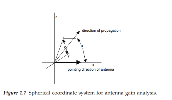
where $P_T$ and $P_R$ are the transmitted, $T$, and received, $R$, powers, respectively; $G_T$ and $G_R$ the transmitting and receiving antenna gains, respectively; $\lambda$ the wavelength of the electromagnetic wave, $R$ the distance between the antennas, and $g_T(\theta, \phi)$ and $g_R(\theta, \phi)$ the relative directive gains at spherical angles $(\theta, \phi)$ measured from the pointing direction of each antenna (Figure 1.7) with a convenient reference direction for $\phi$. The transmission loss equation is often expressed in decibels:
$$
\begin{gathered}
P_R=P_T\left(\frac{G_T G_R \lambda^2}{(4 \pi R)^2}\right) g_T(\theta, \phi) g_R\left(\theta^{\prime}, \phi^{\prime}\right) \
\mathbf{P}{\mathbf{R}}=10 \log {10}\left(P_R\right)=10 \log {10}\left(\frac{P_T G_T g_T G_R g_R \lambda^2}{(4 \pi R)^2}\right) \ \mathbf{P}{\mathbf{R}}=\mathbf{P}{\mathbf{T}}+\mathbf{G}{\mathbf{T}}+\mathbf{g}{\mathbf{T}}+\mathbf{G}{\mathbf{R}}+\mathbf{g}{\mathbf{R}}+20 \log {10}(\lambda)-20 \log {10}(R)-22 \ \mathbf{L}=\mathbf{P}{\mathbf{T}}-\mathbf{P}{\mathbf{R}}=-\left(\mathbf{G}{\mathbf{T}}+\mathbf{g}{\mathbf{T}}+\mathbf{G}{\mathbf{R}}+\mathbf{g}{\mathbf{R}}+20 \log {10}(\lambda)-20 \log {10}(R)-22\right) \ \mathbf{L}{\mathbf{B}}=-\left(20 \log {10}(\lambda)-20 \log {10}(R)-22\right)
\end{gathered}
$$
where $L$ is the transmission loss, $\mathbf{L}_{\mathbf{B}}$ the basic transmission loss; the powers, $\mathbf{P}$, are in decibels, the antenna gains, $\mathbf{G}$, in decibels relative to an isotropic antenna ( $\mathrm{dBi}$ ), and the range (or distance) and wavelength are in the same units of length. The basic transmission loss is just the free space loss, that is, the loss between two isotropic antennas. If the unit of power is a watt, the power is in decibel watt (dBW). In many applications, it is convenient to mix some of the units. For antennas pointed toward each other to maximize their gains, $g_T(\theta, \phi)=1$ and $g_R(\theta, \phi)=1$; for $\lambda=c / f$ with frequency, $f$, in gigaHertz and $c \approx 3 \times 10^8 \mathrm{~m} / \mathrm{s}$ the speed of light. For range in kilometers and for received power expressed in milliwatts and transmitter power in watts, the transmission equation becomes:
$$
\mathbf{P}{\mathbf{R}}=\mathbf{P}{\mathbf{T}}+\mathbf{G}{\mathbf{T}}+\mathbf{G}{\mathbf{R}}-20 \log {10}(f)-20 \log {10}(R)-62.4 \mathrm{dBm}
$$
The directive gain of an antenna, $D$, is:
$$
e D(\theta, \phi)=G g(\theta, \phi)
$$
where $e$ is the antenna efficiency. The directive gain of an antenna describes the ability of the antenna to concentrate the energy radiated by the antenna in a specified direction. It is the ratio of the energy propagating in the specified direction to the energy that would have been transmitted in that direction by an isotropic antenna. ${ }^7$ For an isotropic antenna, the energy transmitted per unit solid angle is $P_{\mathrm{T}} / 4 \pi$. The radiated power flux density (the magnitude of the time average Poynting vector, the radiated power per unit area per unit solid angle) at a distance $R$ from an isotropic antenna is $S=P_T / 4 \pi R^2$. The power collected by a receiving antenna is the power flux density times the effective area of the receiving antenna normal to the direction of propagation, $A_e$. The gain of a receiving antenna is related to $A_e$ by $G_R=4 \pi / \lambda^2 A_e$. The free space loss between the two antennas is then given by $\lambda^2 /(4 \pi R)^2$. The gain of an antenna differs from the directive gain for that
电子工程代写|通讯系统代写Communication System代考|Antenna beamwidth
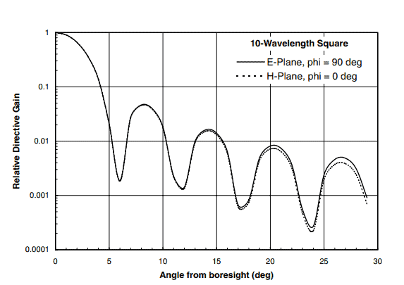
The directive gain of an antenna describes its antenna pattern, that is, the variation in directive gain about pointing direction of the antenna. Figure $1.9$ presents the principal plane patterns for a 10-wavelength square-aperture antenna. The beamwidth of an antenna is the angle enclosing the main lobe or twice the angle between the boresight direction and a reference power on the main lobe of the antenna pattern. Several different beamwidth definitions are in use: the half-power beamwidth, the tenth-power beamwidth, and the beamwidths between nulls. The half-power beamwidth, $\Theta_H$, for this antenna is $5.06^{\circ}$. The maximum directive gain or directivity may be approximated by:
$$
D_0=D(0,0) \approx \frac{4 \pi}{\Theta_{H 1} \Theta_{H 2}}
$$
where the half-power beamwidths for the two principal planes are in radians. For the 10-wavelength square aperture, the maximum directive gain is approximately 1610 or $32 \mathrm{dBi}$. The theoretical directivity for this antenna is $31 \mathrm{dBi}$
通讯系统代写
电子工程代写通讯系统代写COMMUNICATION SYSTEM代 考|TYPES OF SYSTEMS
无线系统使用天线来发送和接收电磁波。天线可以是线天线、孔径天线、线阵列或孔径天线、或反射器天线,其中能量通过天线的组合馈送到反射器。通常天线被 天线罩覆盖或封闭以保护它免受天气影响。根据天线和天线罩的设计,一些天线比其他天线更容易受到天线或天线置上的雨水或湿雪或两者兼而有之的增益损失。 用于收集数据的地面终端天线如图所示 $1.2$ 到图1.6可能会遭受超过的信号减少 $24 \mathrm{~dB}$ 由于反射器上的湿雪。 ${ }^4$ 在编制图中显示的统计数据之前,从数据中审查了雪 事件。天线反射器上的雨水和天线帻源上的天线置可能会产生额外的 $5 \mathrm{~dB}$ 或在高降雨率下损失更多。 ${ }^5$ 这些图中显示的 EDF没有针对雨水对天线的影响进行校正。
在哪里 $P_T$ 和 $P_R$ 是传输的, $T$ ,并收到, $R$, 权力, 分别; $G_T$ 和 $G_R$ 分别为发射和接收天线增益; $\lambda$ 电磁波的波长, $R$ 天线之间的距离,和 $g_T(\theta, \phi)$ 和 $g_R(\theta, \phi)$ 球面角的 相对方向增益 $(\theta, \phi)$ 从每个天线的指向方向测量 Figure 1.7有一个方便的参考方向 $\phi$. 传输损耗方程通常以分贝表示:
$$
P_R=P_T\left(\frac{G_T G_R \lambda^2}{(4 \pi R)^2}\right) g_T(\theta, \phi) g_R\left(\theta^{\prime}, \phi^{\prime}\right) \mathbf{P R}=10 \log 10\left(P_R\right)=10 \log 10\left(\frac{P_T G_T g_T G_R g_R \lambda^2}{(4 \pi R)^2}\right) \mathbf{P R}=\mathbf{P T}+\mathbf{G T}+\mathbf{g T}+\mathbf{G R}+\mathbf{g}+20 \log 10(\lambda)-
$$
在哪里 $L$ 是传输损耗, $\mathbf{L}{\mathrm{B}}$ 基本传输损耗;权力, $\mathbf{P}$, 以分贝为单位, 天线增益, $\mathbf{G}$, 相对于各向同性天线的分贝 $\$ \mathrm{dBi} \$$, 和范围ordistance和波长的长度单位相同。基 本传输损耗就是目由空间损耗,即两个各向同性天线之间的损耓。如果功率单位是瓦特,则功率为分贝瓦特 $d B W$. 在许多应用中,混合一些单元很方便。对于指向 彼此以最大化其增益的天线, $g_T(\theta, \phi)=1$ 和 $g_R(\theta, \phi)=1$; 为了 $\lambda=c / f$ 随着频率, $f$, 千兆赫和 $c \approx 3 \times 10^8 \mathrm{~m} / \mathrm{s}$ 光的速度。对于以千米为单位的范围和以室瓦表 示的接收功率和以瓦特表示的发射机功率,传输方程变为: $$ \mathbf{P R}=\mathbf{P T}+\mathbf{G T}+\mathbf{G R}-20 \log 10(f)-20 \log 10(R)-62.4 \mathrm{dBm} $$ 天线的方向性增益, $D$ ,是: $$ e D(\theta, \phi)=G g(\theta, \phi) $$ 在哪里 $e$ 是天线效率。天线的定向增益描述了天线将天线辐射的能量集中在指定方向的能力。它是在指定方向上传播的能量与各向同性天线在该方向上传输的能量 之比。 ${ }^7$ 对于各向同性天线,每单位立体角发射的能量为 $P{\mathrm{T}} / 4 \pi$. 辐射功率通量密度
themagnitudeofthetimeaveragePoyntingvector, theradiatedpowerperunitareaperunitsolidangle在远处 $R$ 从各向同性天线是 $S=P_T / 4 \pi R^2$. 接收天线 收集的功率是功率通量密度乘以垂直于传播方向的接收天线的有效面积, $A_e$. 接收天线的增益与 $A_e$ 经过 $G_R=4 \pi / \lambda^2 A_e$. 两个天线之间的自由空间损耗由下式给出 $\lambda^2 /(4 \pi R)^2$. 天线的增益不同于该天线的定向增益
电子工程代写通讯系统代写COMMUNICATION SYSTEM代 考|ANTENNA BEAMWIDTH
天线的指向增益描述了它的天线方向图,即指向增益关于天线指向的变化。数字 $1.9$ 展示了 10 波长方孔径天线的主平面方向图。天线的波束宽度是围绕主龵的角 度,或者是视轴方向与天线方向图主瓣上的参考功率之间的角度的两倍。使用了几种不同的波束宽度定义:半功率波束宽度、10次功率波束宽度和零点之间的波束 宽度。半功率波束宽度, $\Theta_H$, 因为这个天线是 $5.06^{\circ}$. 最大定向增益或方向性可以近似为:
$$
D_0=D(0,0) \approx \frac{4 \pi}{\Theta_{H 1} \Theta_{H 2}}
$$
其中两个主平面的半功率波束宽度以弧度为单位。对于 10 波长方孔,最大定向增益约为 1610 或 $32 \mathrm{dBi}$. 该天线的理论方向性为 $31 \mathrm{dBi}$

电子工程代写|通讯系统代写COMMUNICATION SYSTEM代考 请认准UprivateTA™. UprivateTA™为您的留学生涯保驾护航。
微观经济学代写
微观经济学是主流经济学的一个分支,研究个人和企业在做出有关稀缺资源分配的决策时的行为以及这些个人和企业之间的相互作用。my-assignmentexpert™ 为您的留学生涯保驾护航 在数学Mathematics作业代写方面已经树立了自己的口碑, 保证靠谱, 高质且原创的数学Mathematics代写服务。我们的专家在图论代写Graph Theory代写方面经验极为丰富,各种图论代写Graph Theory相关的作业也就用不着 说。
线性代数代写
线性代数是数学的一个分支,涉及线性方程,如:线性图,如:以及它们在向量空间和通过矩阵的表示。线性代数是几乎所有数学领域的核心。
博弈论代写
现代博弈论始于约翰-冯-诺伊曼(John von Neumann)提出的两人零和博弈中的混合策略均衡的观点及其证明。冯-诺依曼的原始证明使用了关于连续映射到紧凑凸集的布劳威尔定点定理,这成为博弈论和数学经济学的标准方法。在他的论文之后,1944年,他与奥斯卡-莫根斯特恩(Oskar Morgenstern)共同撰写了《游戏和经济行为理论》一书,该书考虑了几个参与者的合作游戏。这本书的第二版提供了预期效用的公理理论,使数理统计学家和经济学家能够处理不确定性下的决策。
微积分代写
微积分,最初被称为无穷小微积分或 “无穷小的微积分”,是对连续变化的数学研究,就像几何学是对形状的研究,而代数是对算术运算的概括研究一样。
它有两个主要分支,微分和积分;微分涉及瞬时变化率和曲线的斜率,而积分涉及数量的累积,以及曲线下或曲线之间的面积。这两个分支通过微积分的基本定理相互联系,它们利用了无限序列和无限级数收敛到一个明确定义的极限的基本概念 。
计量经济学代写
什么是计量经济学?
计量经济学是统计学和数学模型的定量应用,使用数据来发展理论或测试经济学中的现有假设,并根据历史数据预测未来趋势。它对现实世界的数据进行统计试验,然后将结果与被测试的理论进行比较和对比。
根据你是对测试现有理论感兴趣,还是对利用现有数据在这些观察的基础上提出新的假设感兴趣,计量经济学可以细分为两大类:理论和应用。那些经常从事这种实践的人通常被称为计量经济学家。
Matlab代写
MATLAB 是一种用于技术计算的高性能语言。它将计算、可视化和编程集成在一个易于使用的环境中,其中问题和解决方案以熟悉的数学符号表示。典型用途包括:数学和计算算法开发建模、仿真和原型制作数据分析、探索和可视化科学和工程图形应用程序开发,包括图形用户界面构建MATLAB 是一个交互式系统,其基本数据元素是一个不需要维度的数组。这使您可以解决许多技术计算问题,尤其是那些具有矩阵和向量公式的问题,而只需用 C 或 Fortran 等标量非交互式语言编写程序所需的时间的一小部分。MATLAB 名称代表矩阵实验室。MATLAB 最初的编写目的是提供对由 LINPACK 和 EISPACK 项目开发的矩阵软件的轻松访问,这两个项目共同代表了矩阵计算软件的最新技术。MATLAB 经过多年的发展,得到了许多用户的投入。在大学环境中,它是数学、工程和科学入门和高级课程的标准教学工具。在工业领域,MATLAB 是高效研究、开发和分析的首选工具。MATLAB 具有一系列称为工具箱的特定于应用程序的解决方案。对于大多数 MATLAB 用户来说非常重要,工具箱允许您学习和应用专业技术。工具箱是 MATLAB 函数(M 文件)的综合集合,可扩展 MATLAB 环境以解决特定类别的问题。可用工具箱的领域包括信号处理、控制系统、神经网络、模糊逻辑、小波、仿真等。