
如果你也在 怎样代写机器学习Machine Learning ACDL2022 这个学科遇到相关的难题,请随时右上角联系我们的24/7代写客服。机器学习Machine Learning是一个致力于理解和建立 “学习 “方法的研究领域,也就是说,利用数据来提高某些任务的性能的方法。机器学习算法基于样本数据(称为训练数据)建立模型,以便在没有明确编程的情况下做出预测或决定。机器学习算法被广泛用于各种应用,如医学、电子邮件过滤、语音识别和计算机视觉,在这些应用中,开发传统算法来执行所需任务是困难的或不可行的。
机器学习Machine Learning程序可以在没有明确编程的情况下执行任务。它涉及到计算机从提供的数据中学习,从而执行某些任务。对于分配给计算机的简单任务,有可能通过编程算法告诉机器如何执行解决手头问题所需的所有步骤;就计算机而言,不需要学习。对于更高级的任务,由人类手动创建所需的算法可能是一个挑战。在实践中,帮助机器开发自己的算法,而不是让人类程序员指定每一个需要的步骤,可能会变得更加有效 。
机器学习Machine Learning代写,免费提交作业要求, 满意后付款,成绩80\%以下全额退款,安全省心无顾虑。专业硕 博写手团队,所有订单可靠准时,保证 100% 原创。 最高质量的机器学习Machine Learning作业代写,服务覆盖北美、欧洲、澳洲等 国家。 在代写价格方面,考虑到同学们的经济条件,在保障代写质量的前提下,我们为客户提供最合理的价格。 由于作业种类很多,同时其中的大部分作业在字数上都没有具体要求,因此机器学习Machine Learning作业代写的价格不固定。通常在专家查看完作业要求之后会给出报价。作业难度和截止日期对价格也有很大的影响。
同学们在留学期间,都对各式各样的作业考试很是头疼,如果你无从下手,不如考虑my-assignmentexpert™!
my-assignmentexpert™提供最专业的一站式服务:Essay代写,Dissertation代写,Assignment代写,Paper代写,Proposal代写,Proposal代写,Literature Review代写,Online Course,Exam代考等等。my-assignmentexpert™专注为留学生提供Essay代写服务,拥有各个专业的博硕教师团队帮您代写,免费修改及辅导,保证成果完成的效率和质量。同时有多家检测平台帐号,包括Turnitin高级账户,检测论文不会留痕,写好后检测修改,放心可靠,经得起任何考验!
想知道您作业确定的价格吗? 免费下单以相关学科的专家能了解具体的要求之后在1-3个小时就提出价格。专家的 报价比上列的价格能便宜好几倍。
我们在计算机Quantum computer代写方面已经树立了自己的口碑, 保证靠谱, 高质且原创的计算机Quantum computer代写服务。我们的专家在机器学习Machine Learning代写方面经验极为丰富,各种机器学习Machine Learning相关的作业也就用不着 说。
机器学习代考_Machine Learning代考_DRL Framework
Generally, the agent uses quality function $Q$ to evaluate the quality of the current policy, which is defined as follows:
$$
Q\left(s_t, a_t\right)=\mathbb{E}\left[R_t+\gamma Q\left(s_{t+1}, a_{t+1}\right)\right]
$$
where $\mathbb{E}$ denotes the expectation value. For a large input space, the $Q$ of each $(s, a)$ pair cannot be stored in a table since many pairs need a large space to store many different values. Thus, DRL uses a neural network as a function approximator to calculate the $Q$ value of each $(s, a$ ) pair (Mnih et al. 2015). The neural network is denoted as $Q\left(s, a \mid \theta^Q\right.$ ) with neural network parameter $\theta Q$. During the training, the agent changes the neural network by updating the neural network parameters with back propagation. The loss function of the back propagation is defined as follows:
$$
L\left(\theta^Q\right)=\mathbb{E}\left[\left(y_t-Q\left(s_t, a_t \mid \theta\right)\right)^2\right],
$$
where
$$
y_t=R\left(s_t, a_t\right)+\gamma Q\left(s_{t+1}, \mu\left(s_{t+1}\right) \mid \theta^Q\right) .
$$
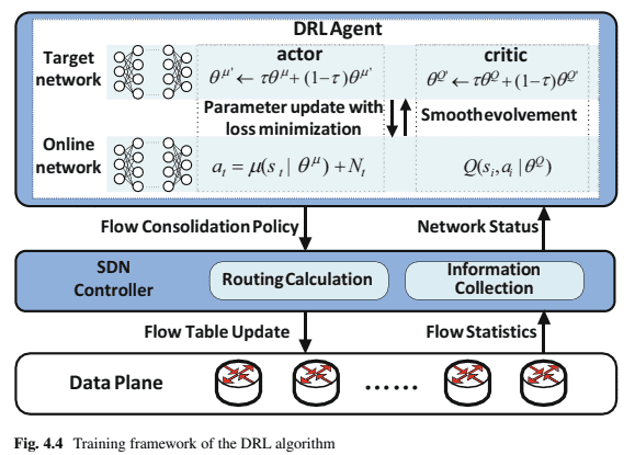
We use DRL to control the link margin ratio. In our design, the action is to decide the link margin ratio, which is a continuous value. A typical way to generate continuous actions in DRL is to use the actor-critic framework (e.g., DDPG (Lillicrap et al. 2015), A3C (Mnih et al. 2016)). The actor-critic framework uses two types of neural networks: actor network and critic network. The critic network is used to evaluate the quality of temporary policy, which can be denoted with $\theta^Q$. The actor network is used to generate actions based on the input state, which can be denoted as $\theta^\mu$. Thus, at any time step, the output action is $a=$ $\mu\left(s \mid \theta^\mu\right)$. The critic network can be trained with Eq. (4.2). The actor network is trained with a gradient value:
$$
\nabla_{\theta^\mu} J=E\left[\nabla_a Q\left(s, a \mid \theta^Q\right) \nabla_{\theta^\mu} \mu\left(s \mid \theta^\mu\right)\right],
$$
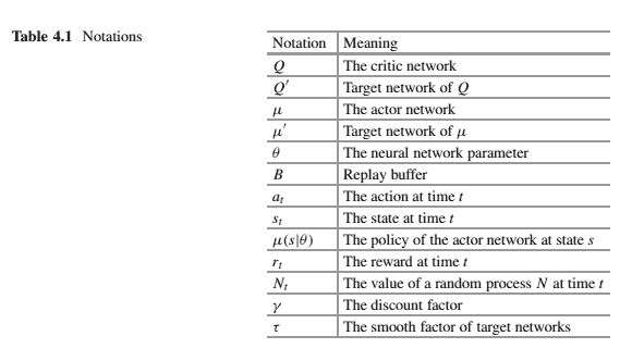
where $J$ is the expected cumulative reward. Table $4.1$ explains the parameters of above equations.
机器学习代考_Machine Learning代考_DRL Implementation Details
The state, action, and reward interfaces in SmartFCT are defined as follows:
State: state is the normalized link utilization and denoted as list $\mathbf{s}_{\mathbf{t}}=\left[s_t^1, s_t^2, \ldots, s_t^L\right]$ at time step $t$, where $L$ is the number of links in the network.
Action: action denotes each link’s margin ratio, which is the output of the actor network added with noise $\epsilon$. The noise is used for policy exploration. We clip the output values from the DRL to $[0,1]$. Action list at time step $t$ is denoted as $\mathbf{a}_{\mathbf{t}}=\left[a_t^1, a_t^2, \ldots, a_t^L\right]$, where $0 \leq a_t^l \leq 1$ and $0 \leq l \leq L$.
Reward: reward is defined as $r_t=D\left[U_l\right]-\lambda C$, where $D\left[U_l\right]$ denotes the number of turned-off/slept links in the network, $C$ denotes the number of flows whose FCT are violated, and $\lambda$ denotes the weight of FCT violation punishment.
Algorithm 5 shows the DRL algorithm of SmartFCT. In the algorithm, lines 1-3 initialize the elements of the DRL algorithm. Line 4 starts the training episodes. Line 5 initializes the algorithm’s random exploration process. Lines 6-16 describe $T$ steps of training. For step $t$, lines $7-9$ present one step of interaction between the DRL agent and the network environment, and lines 10-15 use the interaction data in the buffer to train the neural networks of the DRL agent.
For the implementation of the neural networks in our DRL algorithm, we use a combination of GRU (Cho et al. 2014) and Feed Forward neural network (FF) (Tahmasebi and Hezarkhani 2011). GRU is a modified version of RNN that is designed to extract time-relevant information from the input data. Compared to LSTM, GRU can achieve similar performance but with less computation cost in our scenario. The input data is first processed by the GRU, and the output of GRU is used as the input of an FF. The output layer of FF is then used as the output layer for the final neural network output. Figure $4.5$ shows the combination of these neural networks. State list $\mathbf{s}=\left[s^1, s^2, \ldots, s^L\right]$ is sent to the input layer of GRU, and $\mathbf{h}=\left[h^1, h^2, \ldots, h^L\right]$ is the hidden state of GRU and serves as the output of GRU and the input of FF.
机器学习代写
机器学习代考MACHINE LEARNING代考_DRL FRAMEWORK
一般情况下,代理使用质量函数 $Q$ 评估当前政策的质量,其定义如下: $$ Q\left(s_t, a_t\right)=\mathbb{E}\left[R_t+\gamma Q\left(s{t+1}, a_{t+1}\right)\right]
$$
在哪里 $E$ 表示期望值。对于大的输入空间, $Q$ 每个 $(s, a)$ pair 不能存储在表中,因为许多 pair 需要很大的空间来存储许多不同的值。因此,DRL使用神经网络作为函 数逼近器来计算 $Q$ 每个的价值 $(s, a)$ 一对 Mnihetal. 2015 . 神经网络表示为 $Q\left(s, a \mid \theta^Q\right)$ 与神经网络参数 $\theta Q$. 在训练期间,代理通过反向传播更新神经网络参数来 改变神经网络。反向传播的损失函数定义如下:
$$
L\left(\theta^Q\right)=\mathbb{E}\left[\left(y_t-Q\left(s_t, a_t \mid \theta\right)\right)^2\right],
$$
在哪里
$$
y_t=R\left(s_t, a_t\right)+\gamma Q\left(s_{t+1}, \mu\left(s_{t+1}\right) \mid \theta^Q\right) .
$$
我们使用 DRL来控制链接边距比率。在我们的设计中,动作是决定链路边距比,它是一个连续的值。在 DRL 中生成连续动作的典型方法是使用 actor-critic框架 e.g., DDPG (Lillicrapetal. 2015, A3CMnihetal. 2016). actor-critic 框架使用两种类型的神经网络: actor network 和 critic network。批评网络用于评估临时政策 的质量,可以表示为 $\theta^Q$. 演员网络用于根据输入状态生成动作,可以表示为 $\theta^\mu$. 因此,在任何时间步,输出动作是 $a=\mu\left(s \mid \theta^\mu\right)$. 评论网络可以用等式进行训练。 4.2. 演员网络使用梯度值进行训练:
$$
\nabla_{\theta^\mu} J=E\left[\nabla_a Q\left(s, a \mid \theta^Q\right) \nabla_{\theta^\mu} \mu\left(s \mid \theta^\mu\right)\right],
$$
在哪里 $J$ 是预期的甸积奖励。桌子 $4.1$ 解释上述等式的参数。
机器学习代考MACHINE LEARNING代考_DRL IMPLEMENTATION DETAILS SmartFCT
中的state、action、reward接口定义如下: 状态: 状态是归一化的链路利用率,表示为列表 $s{\mathbf{t}}=\left[s_t^1, s_t^2, \ldots, s_t^L\right]$ 在时间步 $t$ ,在哪里 $L$ 是网絡中的链接数。
action: action表示每个链接的margin ratio,是actor网络加入noise后的输出 $\epsilon$. 噪音用于政策探索。我们将 DRL 的输出值裁剪为 $[0,1]$. 时间步的动作列表 $t$ 表示为 $\mathbf{a}_{\mathbf{t}}=\left[a_t^1, a_t^2, \ldots, a_t^L\right]$, 在哪里 $0 \leq a_t^l \leq 1$ 和 $0 \leq l \leq L$.
奖励:奖励定义为 $r_t=D\left[U_l\right]-\lambda C$ ,在哪里 $D\left[U_l\right]$ 表示网络中关闭/休眠链路的数量, $C$ 表示违反 $\mathrm{FCT}$ 的流的数量,并且 $\lambda$ 表示 FCT 违规惩罚的权重。
算法 5 显示了 SmartFCT 的 DRL 算法。在该算法中,第 1-3 行初始化 DRL 算法的元䋤。第 4 行开始训练片段。第 5 行初始化算法的随机探索过程。第 6-16行描述 $T$ 训 练的步骤。对于步䝨t, 线条 $7-9$ 展示了 DRL代理与网络环境交互的一个步骤,第 10-15行使用缓冲区中的交互数据来训练 DRL代理的神经网絡。
为了在我们的 DRL 算法中实现神经网络,我们使用 GRU 的组合Choetal. 2014和前帻神经网络FF TahmasebiandHezarkhani2011. GRU 是 RNN 的修改版本, 旨在从输入数据中提取与时间相关的信息。与 LSTM 相比,GRU 在我们的场景中可以实现类似的性能,但计算成本更低。输入数据首先由 GRU 处理,GRU 的输出用 作 FF 的输入。然后将FF的输出层作为最终神经网络输出的输出层。数字 $4.5$ 显示了这些神经网络的组合。状态表 $s=\left[s^1, s^2, \ldots, s^L\right]$ 被送到 $G R U$ 的输入层,并且 $\mathbf{h}=\left[h^1, h^2, \ldots, h^L\right]$ 是GRU的隐藏状态,作为 $\mathrm{GRU}$ 的输出和FF的输入。

机器学习代考_Machine Learning代考_ 请认准UprivateTA™. UprivateTA™为您的留学生涯保驾护航。
微观经济学代写
微观经济学是主流经济学的一个分支,研究个人和企业在做出有关稀缺资源分配的决策时的行为以及这些个人和企业之间的相互作用。my-assignmentexpert™ 为您的留学生涯保驾护航 在数学Mathematics作业代写方面已经树立了自己的口碑, 保证靠谱, 高质且原创的数学Mathematics代写服务。我们的专家在图论代写Graph Theory代写方面经验极为丰富,各种图论代写Graph Theory相关的作业也就用不着 说。
线性代数代写
线性代数是数学的一个分支,涉及线性方程,如:线性图,如:以及它们在向量空间和通过矩阵的表示。线性代数是几乎所有数学领域的核心。
博弈论代写
现代博弈论始于约翰-冯-诺伊曼(John von Neumann)提出的两人零和博弈中的混合策略均衡的观点及其证明。冯-诺依曼的原始证明使用了关于连续映射到紧凑凸集的布劳威尔定点定理,这成为博弈论和数学经济学的标准方法。在他的论文之后,1944年,他与奥斯卡-莫根斯特恩(Oskar Morgenstern)共同撰写了《游戏和经济行为理论》一书,该书考虑了几个参与者的合作游戏。这本书的第二版提供了预期效用的公理理论,使数理统计学家和经济学家能够处理不确定性下的决策。
微积分代写
微积分,最初被称为无穷小微积分或 “无穷小的微积分”,是对连续变化的数学研究,就像几何学是对形状的研究,而代数是对算术运算的概括研究一样。
它有两个主要分支,微分和积分;微分涉及瞬时变化率和曲线的斜率,而积分涉及数量的累积,以及曲线下或曲线之间的面积。这两个分支通过微积分的基本定理相互联系,它们利用了无限序列和无限级数收敛到一个明确定义的极限的基本概念 。
计量经济学代写
什么是计量经济学?
计量经济学是统计学和数学模型的定量应用,使用数据来发展理论或测试经济学中的现有假设,并根据历史数据预测未来趋势。它对现实世界的数据进行统计试验,然后将结果与被测试的理论进行比较和对比。
根据你是对测试现有理论感兴趣,还是对利用现有数据在这些观察的基础上提出新的假设感兴趣,计量经济学可以细分为两大类:理论和应用。那些经常从事这种实践的人通常被称为计量经济学家。
Matlab代写
MATLAB 是一种用于技术计算的高性能语言。它将计算、可视化和编程集成在一个易于使用的环境中,其中问题和解决方案以熟悉的数学符号表示。典型用途包括:数学和计算算法开发建模、仿真和原型制作数据分析、探索和可视化科学和工程图形应用程序开发,包括图形用户界面构建MATLAB 是一个交互式系统,其基本数据元素是一个不需要维度的数组。这使您可以解决许多技术计算问题,尤其是那些具有矩阵和向量公式的问题,而只需用 C 或 Fortran 等标量非交互式语言编写程序所需的时间的一小部分。MATLAB 名称代表矩阵实验室。MATLAB 最初的编写目的是提供对由 LINPACK 和 EISPACK 项目开发的矩阵软件的轻松访问,这两个项目共同代表了矩阵计算软件的最新技术。MATLAB 经过多年的发展,得到了许多用户的投入。在大学环境中,它是数学、工程和科学入门和高级课程的标准教学工具。在工业领域,MATLAB 是高效研究、开发和分析的首选工具。MATLAB 具有一系列称为工具箱的特定于应用程序的解决方案。对于大多数 MATLAB 用户来说非常重要,工具箱允许您学习和应用专业技术。工具箱是 MATLAB 函数(M 文件)的综合集合,可扩展 MATLAB 环境以解决特定类别的问题。可用工具箱的领域包括信号处理、控制系统、神经网络、模糊逻辑、小波、仿真等。