物理代写|Physics6561 Electrodynamics

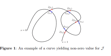
Suppose $\mathbf{r}(s), s \in[0,1]$, is a smooth closed curve in the $x-y$ plane. What are the possible values of the following double integral?
$$
\mathcal{J}=\int_0^1 d s \int_{s^{+}}^1 d t \hat{\mathbf{z}} \cdot \dot{\mathbf{r}}(s) \times \dot{\mathbf{r}}(t) \delta^2(\mathbf{r}(s)-\mathbf{r}(t))
$$

The last factor in the integrand is standard shorthand for the product of two Dirac deltas:
$$
\delta^2(\mathbf{r}(s)-\mathbf{r}(t))=\delta(x(s)-x(t)) \delta(y(s)-y(t))
$$

Delta function forces us to evaluate integrand when $\mathbf{r}(s)=\mathbf{r}(t)$. However integrand $\hat{\mathbf{z}} \cdot \dot{\mathbf{r}}(s) \times \dot{\mathbf{r}}(t)$ yields zero when $\hat{\mathbf{r}}(\mathbf{s})=\hat{\dot{\mathbf{r}}}(\mathbf{t})$, so if we allow $t=s$ the integrand is zero while delta function is non-zero and the integral is not well-defined. Note that this scenario was excluded in the second edition of problem set due to range of $t, t \in(s, 1]$. Thus, the only possibility for finding a non-zero answer is to have points that are intersecting but velocities are not pointing along the same direction, as shown below.
Let’s evaluate integral for these curves. One subtlety is $\delta$-functions are functions of $x(s)-x(t), y(s)-y(t)$, so we need to take into account Jacobian of transformations between $s, t$ and $x(s), x(t)$ (similarly for $y(t), y(s)$ ). To be more concrete, let’s digress for a moment and try to evaluate following integral. First, let’s find the one-dimensional integral:
$$
\begin{gathered}
\int d x \delta(f(x)) g(x) \
f(x)=0 \quad \Rightarrow \quad x=x_0 \
f(x) \approx f\left(x_0\right)+f^{\prime}\left(x_0\right)\left(x-x_0\right)=f^{\prime}\left(x_0\right)\left(x-x_0\right) \
\int d x \delta\left(f^{\prime}\left(x_0\right)\left(x-x_0\right)\right) g(x)=\int d x \frac{\delta\left(x-x_0\right)}{\left|f^{\prime}\left(x_0\right)\right|} g(x)=\frac{g\left(x_0\right)}{\left|f\left(x_0\right)\right|}
\end{gathered}
$$
Now let’s consider a two-dimensional example.
$$
\int d s d t \delta\left(f_1(s, t)\right) \delta\left(f_2(s, t)\right) g(s, t)
$$
Let’s assume $f_1\left(s_0, t_0\right)=0, f_2\left(s_0, t_0\right)=0$, and there is a one-to-one relationships between $(s, t)$ and $\left(f_1, f_2\right)$ in the vicinity of $\left(s_0, t_0\right)$. Then, using change of variables theorem,
$$
\begin{aligned}
& \int d s d t \delta\left(f_1(s, t)\right) \delta\left(f_2(s, t)\right) g(s, t) \
& =\int d f_1 d f_2 \frac{1}{\left|\begin{array}{ll}
\partial_s f_1 & \partial_t f_1 \
\partial_s f_2 & \partial_t f_2
\end{array}\right|} \delta\left(f_1\right) \delta\left(f_2\right) g(s, t)= \
& \left.\frac{g(s, t)}{\left|\begin{array}{ll}
\partial_s f_1 & \partial_t f_1 \
\partial_s f_2 & \partial_t f_2
\end{array}\right|}\right|_{\left(s_0, t_0\right)}=\frac{g\left(s_0, t_0\right)}{\left|\partial_s f_1\left(s_0, t_0\right) \partial_t f_2\left(s_0, t_0\right)-\partial_t f_1\left(s_0, t_0\right) \partial_s f_1\left(s_0, t_0\right)\right|}
\end{aligned}
$$

In an effort to find the simplest shape for a given knotted topology of a loop of string, mathematicians have considered minimizing an energy model where all pairs of line elements $d \mathbf{r}_1$ and $d \mathbf{r}_2$ of the string interact ‘electrostatically’:
$$
d U=\frac{\left|d \mathbf{r}_1\right|\left|d \mathbf{r}_2\right|}{\left|\mathbf{r}_1-\mathbf{r}_2\right|^2}
$$
E\&M was never their strong suit, so we forgive them the exponent 2 in their Coulomb’s law! The total energy has the form of a double integral:
$$
U=\oint d s \oint d t\left(\frac{|\dot{\mathbf{r}}(s)||\dot{\mathbf{r}}(t)|}{|\mathbf{r}(s)-\mathbf{r}(t)|^2}-\frac{1}{(s-t)^2}\right) .
$$
The second term in the integrand, which does not depend on the shape of the knot, is needed to make the expression finite. As physicists we admire the fact that this $U$ is invariant with respect to translations and rotations of the knot. And thanks to that exponent 2, we see that it is even invariant with respect to changes in scale. Show that invariance extends to all elements of the group of conformal transformations by verifying it for Kelvin inversions.

We need to verify that the integrand is invariant under inversions:
$$
\begin{aligned}
\mathbf{r} \rightarrow \mathbf{r}^{\prime} & =\frac{\mathbf{r}}{\mathbf{r} \cdot \mathbf{r}} \
\dot{\mathbf{r}}^{\prime}(t) & =\frac{\dot{\mathbf{r}}(t)}{\mathbf{r}(t) \cdot \mathbf{r}(t)}-\frac{2 \mathbf{r}(t)[\mathbf{r}(t) \cdot \dot{\mathbf{r}}(t)]}{(\mathbf{r}(t) \cdot \mathbf{r}(t))^2} \
\left|\dot{\mathbf{r}}^{\prime}(t)\right|^2 & =\frac{\dot{\mathbf{r}}(t) \cdot \dot{\mathbf{r}}(t)}{(\mathbf{r} \cdot \mathbf{r})^2}+\frac{4(\dot{\mathbf{r}} \cdot \mathbf{r})^2}{(\mathbf{r} \cdot \mathbf{r})^3}-\frac{4(\dot{\mathbf{r}} \cdot \mathbf{r})^2}{(\mathbf{r} \cdot \mathbf{r})^3}=\frac{\dot{\mathbf{r}}(t) \cdot \dot{\mathbf{r}}(t)}{(\mathbf{r} \cdot \mathbf{r})^2}
\end{aligned}
$$
Also for denominator goes as:
$$
\begin{aligned}
& \mathbf{r}(s)-\mathbf{r}(t) \rightarrow \frac{\mathbf{r}(s)}{\mathbf{r}(s) \cdot \mathbf{r}(s)}-\frac{\mathbf{r}(t)}{\mathbf{r}(t) \cdot \mathbf{r}(t)} \
& \Rightarrow \quad|\mathbf{r}(s)-\mathbf{r}(t)|^2 \rightarrow \frac{1}{\mathbf{r}(s) \cdot \mathbf{r}(s)}+\frac{1}{\mathbf{r}(t) \cdot \mathbf{r}(t)}-\frac{2 \mathbf{r}(s) \cdot \mathbf{r}(t)}{\mathbf{r}(t) \cdot \mathbf{r}(t) \mathbf{r}(s) \cdot \mathbf{r}(s)} \
& =\frac{(\mathbf{r}(s)-\mathbf{r}(t))^2}{\mathbf{r}(t) \cdot \mathbf{r}(t) \mathbf{r}(s) \cdot \mathbf{r}(s)}
\end{aligned}
$$
Note that using this equation, we can find again (1.3) by setting $t \rightarrow s+\delta s$ and taking the limit.
Combining these two result, we find invariance of the total energy:
$$
\frac{|\dot{\mathbf{r}}(s)||\dot{\mathbf{r}}(t)|}{|\mathbf{r}(s)-\mathbf{r}(t)|^2} \rightarrow \frac{\frac{|\dot{\mathbf{r}}(s)|}{\mathbf{r}^2(s)} \frac{|\dot{\mathbf{r}}(t)|}{\mathbf{r}^2(t)}}{\frac{\mathbf{r}(s)-\left.\mathbf{r}(t)\right|^2}{\mathbf{r}^2(t) \mathbf{r}^2(s)}}=\frac{|\dot{\mathbf{r}}(s)||\dot{\mathbf{r}}(t)|}{|\mathbf{r}(s)-\mathbf{r}(t)|^2}
$$
Which shows invariance under inversion at origin.