MY-ASSIGNMENTEXPERT™可以为您提供lse.ac.uk ST308 Bayesian Analysis贝叶斯分析课程的代写代考和辅导服务!
这是伦敦政经学校贝叶斯分析课程的代写成功案例。

ST308课程简介
This course is available on the BSc in Actuarial Science, BSc in Business Mathematics and Statistics, BSc in Data Science, BSc in Mathematics with Economics and BSc in Mathematics, Statistics and Business. This course is available as an outside option to students on other programmes where regulations permit and to General Course students.
Teaching
This course will be delivered through a combination of classes, lectures, and Q&A sessions, totalling a minimum of 29 hours across the Lent Term. This course does not include a reading week and will be concluded by the end of week 10 of Lent Term.
Prerequisites
Students must have completed one of the following two combinations of courses: (a) ST102 and MA100, or (b) MA107 and ST109 and EC1C1. Equivalent combinations may be accepted at the lecturer’s discretion. ST202 is also recommended.
Previous programming experience is not required but students who have no previous experience in R must complete an online pre-sessional R course from the Digital Skills Lab before the start of the course (https://moodle.lse.ac.uk/course/view.php?id=7745)
ST308 Bayesian Analysis HELP(EXAM HELP, ONLINE TUTOR)
(a) Using the following control parameters, run the optimal-k function to search for the optimal number of topics. Be sure to set the “max.k” parameter equal to 30 .
$$
\text { control <- list (burnin }=500 \text {, iter }=1000, \text { keep }=100 \text {, seed }=46 \text { ) }
$$
(b) Plot the results of the optimal-k function. What does this plot suggest about the number of topics in the text?
(c) Run LDA on the document-term matrix using the optimal value of $\mathrm{k}$. Print out the top 10 words for each of the $\mathrm{k}$ topics. Comment on the results and their plausibility. What does each topic seem to represent?
The first model we will fit to the contraceptives data is a varying-intercept logistic regression model, where the intercept varies by district.
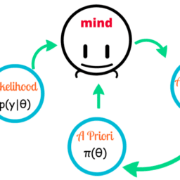
Prior distribution:
$\beta_{0 j} \sim N\left(\mu_0, \sigma_0\right)$, with $\mu_0 \sim N(0,100)$ and $\sigma_0 \sim \operatorname{Exponential}(.1)$
$\beta_1 \sim N(0,100), \beta_2 \sim N(0,100), \beta_3 \sim N(0,100)$
Model for data:
$$
\begin{aligned}
& Y_{i j} \sim \operatorname{Bernoulli}\left(p_{i j}\right) \
& \text { logit } p_{i j}=\beta_{0 j}+\beta_1 * \text { urban }+\beta_2 * \text { living-children }+\beta_3 * \text { age-mean }
\end{aligned}
$$
where $Y_{i j}$ is 1 if woman $i$ in district $j$ uses contraception, and 0 otherwise, and where $i=1, \ldots, N$ and $j=1, \ldots, J$ ( $N$ is the number of observations in the data, and $J$ is the number of districts). The above notation assumes $N(\mu, \sigma)$ is a normal distribution with mean $\mu$ and standard deviation $\sigma$. Also, the above notation assumes $\operatorname{Exponential}(\lambda)$ has mean $1 / \lambda$. These are consistent with the parameterizations in Stan.
After you read the train and test data into $\mathrm{R}$, the following code will help with formatting:
# convert everything to numeric
for (i in $1:$ ncol(train)) {
$\operatorname{train}[, i]<-$ as. numeric(as. character $(\operatorname{train}[, i]))$
test $[, i]<-$ as. numeric(as.character (test $[, i])$ )
}
# map district 61 to 54 (so that districts are in order)
train_bad_indices <- which(train $\$$ district $==61$ )
train[train_bad_indices, 1] <- 54
test_bad_indices $<-$ which(test $\$$ district $==61$ )
test [test_bad_indices, 1] <- 54
(a) To verify the procedure, simulate binary response data (using the rbinom function) assuming the following parameter values (and using the existing features and district information from the training data):
mu_beta_0 02
sigma_beta_0 $=1$
set.seed $(123) \quad$ to ensure the next line is common to everyone
beta_0 $=$ rnorm $(n=60$, mean=mu_beta_0, sd=sigma_beta_0 $)$
beta_1 $=4$
beta_2 $=-3$
beta_3 $=-2$
(b) Fit the varying-intercept model specified above to your simulated data
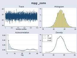
(c) Plot the trace plots of the MCMC sampler for the parameters $\mu_{\beta_0}, \sigma_{\beta_0}, \beta_1, \beta_2, \beta_3$. Does it look like the samplers converged?
(d) Plot histograms of the posterior distributions for the parameters $\beta_{0,10}, \beta_{0,20} \ldots \beta_{0,60}$. Are the actual parameters that you generated contained within these posterior distributions?
We now fit our model to the actual data.
(e) Fit the varying-intercept model to the real train data. Make sure to set a seed at 46 within the Stan function, to ensure that you will get the same results if you fit your model correctly.
(f) Check the convergence by examining the trace plots, as you did with the simulated data.
(g) Based on the posterior means, women belonging to which district are most likely to use contraceptives? Women belonging to which district are least likely to use contraceptives?
(h) What are the posterior means of $\mu_{\beta_0}$ and $\sigma_{\beta_0}$ ? Do these values offer any evidence in support of or against the varying-intercept model?
In the next model we will fit to the contraceptives data is a varying-coefficients logistic regression model, where the coefficients on living-children, age-mean and urban vary by district:
Prior distribution:
$\beta_{0 j} \sim N\left(\mu_0, \sigma_0\right)$, with $\mu_0 \sim N(0,100)$ and $\sigma_0 \sim \operatorname{Exponential}(0.1)$
$\beta_{1 j} \sim N\left(0, \sigma_1\right)$, with $\sigma_1 \sim \operatorname{Exponential}(0.1)$
$\beta_{2 j} \sim N\left(0, \sigma_2\right)$, with $\sigma_2 \sim \operatorname{Exponential}(0.1)$
$\beta_{3 j} \sim N\left(0, \sigma_3\right)$, with $\sigma_3 \sim \operatorname{Exponential}(0.1)$
Model for data:
$Y_{i j} \sim \operatorname{Bernoulli}\left(p_{i j}\right)$
$\operatorname{logit} p_{i j}=\beta_{0 j}+\beta_{1 j}$ urban $+\beta_{2 j}$ age-mean $+\beta_{3 j}$ living-children
where $i=1, \ldots, N$ and $j=1, \ldots, J$ ( $N$ is the number of observations in the data, and $J$ is the number of districts).
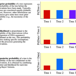
(a) Fit the model to the real data. For each of the three coefficients to the predictors, plot vertical segments corresponding to the $95 \%$ central posterior intervals for the coefficient within each district. Thus you should have 60 parallel segments on each graph. If the segments are overlapping on the vertical scale, then the model fit suggests that the coefficient does not differ by district. What do you conclude from these graphs?
(b) Use all of the information you’ve gleaned thus far to build a final Bayesian logistic regression classifier on the train set. Then, use your model to make predictions on the test set. Report your model’s classification percentage.

MY-ASSIGNMENTEXPERT™可以为您提供LSE.AC.UK ST308 BAYESIAN ANALYSIS贝叶斯分析课程的代写代考和辅导服务!